Lesson 14: Wrap-up of relational data, then
on to iteration with for loops and conditional execution
with if statements
Readings
Required:
Relational data:
If you didn’t get a chance to read it last week, have a look at Chapter 13 in ‘R for Data Science’ by Hadley Wickham & Garrett Grolemund
Iteration:
Chapter 21 in ‘R for Data Science’ by Hadley Wickham & Garrett Grolemund
Other resources:
We will be working through this tutorial developed by the Ocean Health Index Data Science Team
Announcements
Because of the snow day and cancelled class on Tuesday, we have updated the syllabus. We have shifted lectures down and added a make-up lecture the Tuesday after Spring Break * Assignment 7 is still due today * Assignment 8 will not be due until 3/30 * Assignment 9 will be due Tuesday after Spring Break (4/11)
Postdoc Jessi Rick will offer a two-session follow-up workshop during our regular lecture slot on 4/13 and 4/13 about open data science and data sharing/management. This is an optional not-for-credit add-on workshop. More details next week.
Today’s learning objectives
We’ll start by working through a few exercises on using integrating
data from multiple tibbles (using join() functions) and
recap on strategies for successfully integrating relational data. Then
we’ll shift gears to begin exploring the key programming concepts of
iteration and conditional execution.
By the end of today’s and next Tuesday’s class, you should be able to:
- Write a
forloop to repeat operations on different input - Implement
ifandif elsestatements for conditional execution of code
Acknowledgements: Today’s tutorial is adapted (with permission) from the excellent Ocean Health Index Data Science Training.
Recap on relational data
Let’s load the tidyverse and knitr
library(tidyverse)
library(knitr)
The gapminder data
Last class, we used the nycflights13 datasets to explore
the mutating joins. Let’s recap by applying these to a different
dataset. Today we’ll return to the gapminder dataset that
many of you have started exploring in the lab session a few weeks
ago.
The data in the gapminder package is a subset of the Gapminder
dataset, which contains data on the health and wealth of nations
over the past decades. It was pioneered by Hans Rosling, who
is famous for describing the prosperity of nations over time through
famines, wars and other historic events with this beautiful data
visualization in his 2006
TED Talk: The best stats you’ve ever seen:

We will primarily use a subset of the gapminder data included in the
R package gapminder. So first we need to install that
package and load it, along with the tidyverse. Then have a look at the
data in gapminder
library(gapminder) #install.packages("gapminder")

head(gapminder) %>% kable()| country | continent | year | lifeExp | pop | gdpPercap |
|---|---|---|---|---|---|
| Afghanistan | Asia | 1952 | 28.801 | 8425333 | 779.4453 |
| Afghanistan | Asia | 1957 | 30.332 | 9240934 | 820.8530 |
| Afghanistan | Asia | 1962 | 31.997 | 10267083 | 853.1007 |
| Afghanistan | Asia | 1967 | 34.020 | 11537966 | 836.1971 |
| Afghanistan | Asia | 1972 | 36.088 | 13079460 | 739.9811 |
| Afghanistan | Asia | 1977 | 38.438 | 14880372 | 786.1134 |
We can see that this dataset used camelCase (first word lowercase and
capitalize all following words) for its column names. I always use
snake_case (replace spaces with underscores), and it’s going to look
messy to have this inconsistent way of writing variable names. So I’m
going to go ahead and clean these names up before I start working with
the data. I can do this manually with the rename() or
colnames() functions, e.g.
gapminder %>%
  rename("life_exp" = lifeExp, "gdp_per_cap" = gdpPercap)
## # A tibble: 1,704 × 6
## country continent year life_exp pop gdp_per_cap
## <fct> <fct> <int> <dbl> <int> <dbl>
## 1 Afghanistan Asia 1952 28.8 8425333 779.
## 2 Afghanistan Asia 1957 30.3 9240934 821.
## 3 Afghanistan Asia 1962 32.0 10267083 853.
## 4 Afghanistan Asia 1967 34.0 11537966 836.
## 5 Afghanistan Asia 1972 36.1 13079460 740.
## 6 Afghanistan Asia 1977 38.4 14880372 786.
## 7 Afghanistan Asia 1982 39.9 12881816 978.
## 8 Afghanistan Asia 1987 40.8 13867957 852.
## 9 Afghanistan Asia 1992 41.7 16317921 649.
## 10 Afghanistan Asia 1997 41.8 22227415 635.
## # … with 1,694 more rows# Alternative
colnames(gapminder) <- c("country", "continent", "year", "life_exp", "pop", "gdp_per_cap")Alternatively, I can use the clean_names() function from
the janitor package
library(janitor)

clean_names(gapminder)
In the lab section, we have been working with a different subset of
the gapminder dataset that comes with the dslabs package.
Let’s import a chunk of those data that we’ve saved in our class GitHub
repo:
gap_dslabs <- read_csv("https://raw.githubusercontent.com/nt246/NTRES-6100-data-science/main/datasets/gapminder_dslabs_subset_original_names.csv")Exercise
Add the infant mortality and fertility data to our original
gapminder data. Do we have those statistics for all
observations?
In this case, we were lucky that the variables that we wanted to join
the tables by had identical names in the two datasets. Now, let’s
imagine the variables in the dslab version had been named
differently. Run this code to change the variable names:
gap_dslabs_caps <- gap_dslabs %>%
  rename("Country" = country, "Year" = year)
Now add the infant mortality and fertility from the
gap_dslabs_caps to our original `gapminder
data.
Click here for a solution
## When variable names are identical

# Natural join
gapminder %>%
  left_join(gap_dslabs)
## Joining, by = c("country", "year")## # A tibble: 1,704 × 8
## country continent year life_exp pop gdp_per_cap infant_mo…¹ ferti…²
## <chr> <fct> <dbl> <dbl> <int> <dbl> <dbl> <dbl>
## 1 Afghanistan Asia 1952 28.8 8425333 779. NA NA
## 2 Afghanistan Asia 1957 30.3 9240934 821. NA NA
## 3 Afghanistan Asia 1962 32.0 10267083 853. NA NA
## 4 Afghanistan Asia 1967 34.0 11537966 836. NA NA
## 5 Afghanistan Asia 1972 36.1 13079460 740. NA NA
## 6 Afghanistan Asia 1977 38.4 14880372 786. NA NA
## 7 Afghanistan Asia 1982 39.9 12881816 978. NA NA
## 8 Afghanistan Asia 1987 40.8 13867957 852. NA NA
## 9 Afghanistan Asia 1992 41.7 16317921 649. NA NA
## 10 Afghanistan Asia 1997 41.8 22227415 635. NA NA
## # … with 1,694 more rows, and abbreviated variable names ¹infant_mortality,
## # ²fertility# Specifying the variables to join by (useful if some variables mean different things in the two tables you're joining)
gapminder %>%
left_join(gap_dslabs, by = c("country", "year"))## # A tibble: 1,704 × 8
## country continent year life_exp pop gdp_per_cap infant_mo…¹ ferti…²
## <chr> <fct> <dbl> <dbl> <int> <dbl> <dbl> <dbl>
## 1 Afghanistan Asia 1952 28.8 8425333 779. NA NA
## 2 Afghanistan Asia 1957 30.3 9240934 821. NA NA
## 3 Afghanistan Asia 1962 32.0 10267083 853. NA NA
## 4 Afghanistan Asia 1967 34.0 11537966 836. NA NA
## 5 Afghanistan Asia 1972 36.1 13079460 740. NA NA
## 6 Afghanistan Asia 1977 38.4 14880372 786. NA NA
## 7 Afghanistan Asia 1982 39.9 12881816 978. NA NA
## 8 Afghanistan Asia 1987 40.8 13867957 852. NA NA
## 9 Afghanistan Asia 1992 41.7 16317921 649. NA NA
## 10 Afghanistan Asia 1997 41.8 22227415 635. NA NA
## # … with 1,694 more rows, and abbreviated variable names ¹infant_mortality,
## # ²fertility# When variable names are not identical
gapminder %>%
left_join(gap_dslabs_caps, by = c("country" = "Country", "year" = "Year"))## # A tibble: 1,704 × 8
## country continent year life_exp pop gdp_per_cap infant_mo…¹ ferti…²
## <chr> <fct> <dbl> <dbl> <int> <dbl> <dbl> <dbl>
## 1 Afghanistan Asia 1952 28.8 8425333 779. NA NA
## 2 Afghanistan Asia 1957 30.3 9240934 821. NA NA
## 3 Afghanistan Asia 1962 32.0 10267083 853. NA NA
## 4 Afghanistan Asia 1967 34.0 11537966 836. NA NA
## 5 Afghanistan Asia 1972 36.1 13079460 740. NA NA
## 6 Afghanistan Asia 1977 38.4 14880372 786. NA NA
## 7 Afghanistan Asia 1982 39.9 12881816 978. NA NA
## 8 Afghanistan Asia 1987 40.8 13867957 852. NA NA
## 9 Afghanistan Asia 1992 41.7 16317921 649. NA NA
## 10 Afghanistan Asia 1997 41.8 22227415 635. NA NA
## # … with 1,694 more rows, and abbreviated variable names ¹infant_mortality,
## # ²fertility## Note, gap_dslabs doesn't have data for Afghanistan, so the join may not look successful if you just examine the first few lines. Look further down in the tibble.Filtering joins
We’ll review filtering joins and general strategies for combining
information from multiple tables. There are some good examples with the
flights data in R4DS.
Here, we will illustrate with the gapminder data.
Filtering joins match observations in the same way as mutating joins, but affect the observations, not the variables. There are two types:
semi_join(x, y)keeps all observations in x that have a match in y.anti_join(x, y)drops all observations in x that have a match in y.
Semi-joins are useful for matching filtered summary tables back to the original rows.
These functions can be useful when we want to filter based on more
than one variable. If we wanted to grab all the records from Malawi, for
example, we can use filter()
gapminder %>%
  filter(country == "Malawi")
## # A tibble: 12 × 6
## country continent year life_exp pop gdp_per_cap
## <fct> <fct> <int> <dbl> <int> <dbl>
## 1 Malawi Africa 1952 36.3 2917802 369.
## 2 Malawi Africa 1957 37.2 3221238 416.
## 3 Malawi Africa 1962 38.4 3628608 428.
## 4 Malawi Africa 1967 39.5 4147252 496.
## 5 Malawi Africa 1972 41.8 4730997 585.
## 6 Malawi Africa 1977 43.8 5637246 663.
## 7 Malawi Africa 1982 45.6 6502825 633.
## 8 Malawi Africa 1987 47.5 7824747 636.
## 9 Malawi Africa 1992 49.4 10014249 563.
## 10 Malawi Africa 1997 47.5 10419991 692.
## 11 Malawi Africa 2002 45.0 11824495 665.
## 12 Malawi Africa 2007 48.3 13327079 759.However, say we wanted to extract the records from the countries and
years that had the highest fertility rates recorded. It would be harder
to do this with the filter() function in a single step.
This is a case where semi_join() can be useful.
top_fertility <- gap_dslabs %>%
  arrange(-fertility) %>%
  head(10)

gapminder %>%
  semi_join(top_fertility)
## Joining, by = c("country", "year")## # A tibble: 6 × 6
## country continent year life_exp pop gdp_per_cap
## <fct> <fct> <int> <dbl> <int> <dbl>
## 1 Oman Asia 1982 62.7 1301048 12955.
## 2 Rwanda Africa 1962 43 3051242 597.
## 3 Rwanda Africa 1967 44.1 3451079 511.
## 4 Rwanda Africa 1972 44.6 3992121 591.
## 5 Rwanda Africa 1977 45 4657072 670.
## 6 Rwanda Africa 1982 46.2 5507565 882.We notice here that our resulting tibble only include 6 rows, not the
10 we had expected. Upon inspection, we notice that the records from
Yemen are missing. We can confirm that this is because the
gapminder tibble doesn’t include “Yemen” (written this way)
as a country by examining the unique values included in the country
variable.
unique(gapminder$country)## [1] Afghanistan Albania Algeria
## [4] Angola Argentina Australia
## [7] Austria Bahrain Bangladesh
## [10] Belgium Benin Bolivia
## [13] Bosnia and Herzegovina Botswana Brazil
## [16] Bulgaria Burkina Faso Burundi
## [19] Cambodia Cameroon Canada
## [22] Central African Republic Chad Chile
## [25] China Colombia Comoros
## [28] Congo, Dem. Rep. Congo, Rep. Costa Rica
## [31] Cote d'Ivoire Croatia Cuba
## [34] Czech Republic Denmark Djibouti
## [37] Dominican Republic Ecuador Egypt
## [40] El Salvador Equatorial Guinea Eritrea
## [43] Ethiopia Finland France
## [46] Gabon Gambia Germany
## [49] Ghana Greece Guatemala
## [52] Guinea Guinea-Bissau Haiti
## [55] Honduras Hong Kong, China Hungary
## [58] Iceland India Indonesia
## [61] Iran Iraq Ireland
## [64] Israel Italy Jamaica
## [67] Japan Jordan Kenya
## [70] Korea, Dem. Rep. Korea, Rep. Kuwait
## [73] Lebanon Lesotho Liberia
## [76] Libya Madagascar Malawi
## [79] Malaysia Mali Mauritania
## [82] Mauritius Mexico Mongolia
## [85] Montenegro Morocco Mozambique
## [88] Myanmar Namibia Nepal
## [91] Netherlands New Zealand Nicaragua
## [94] Niger Nigeria Norway
## [97] Oman Pakistan Panama
## [100] Paraguay Peru Philippines
## [103] Poland Portugal Puerto Rico
## [106] Reunion Romania Rwanda
## [109] Sao Tome and Principe Saudi Arabia Senegal
## [112] Serbia Sierra Leone Singapore
## [115] Slovak Republic Slovenia Somalia
## [118] South Africa Spain Sri Lanka
## [121] Sudan Swaziland Sweden
## [124] Switzerland Syria Taiwan
## [127] Tanzania Thailand Togo
## [130] Trinidad and Tobago Tunisia Turkey
## [133] Uganda United Kingdom United States
## [136] Uruguay Venezuela Vietnam
## [139] West Bank and Gaza Yemen, Rep. Zambia
## [142] Zimbabwe
## 142 Levels: Afghanistan Albania Algeria Angola Argentina Australia ... ZimbabweSo we would need to make sure country names are consistent in our two
dataframes before proceeding (str_replace() is a good
function for that).
In general, the opposite of semi_join(), the
anti_join() function is good for diagnosing mismatches.
# What records in gapminder are not matched in gap_dslabs
gapminder %>%
  anti_join(gap_dslabs, by = "country")  %>%
  count(country)
## # A tibble: 9 × 2
## country n
## <fct> <int>
## 1 Afghanistan 12
## 2 Korea, Dem. Rep. 12
## 3 Korea, Rep. 12
## 4 Myanmar 12
## 5 Reunion 12
## 6 Sao Tome and Principe 12
## 7 Somalia 12
## 8 Taiwan 12
## 9 Yemen, Rep. 12# What records in gap_dslabs are not matched in gapminder
gap_dslabs %>%
anti_join(gapminder, by = "country") %>%
count(country)## # A tibble: 52 × 2
## country n
## <chr> <int>
## 1 Antigua and Barbuda 10
## 2 Armenia 10
## 3 Aruba 10
## 4 Azerbaijan 10
## 5 Bahamas 10
## 6 Barbados 10
## 7 Belarus 10
## 8 Belize 10
## 9 Bhutan 10
## 10 Brunei 10
## # … with 42 more rowsJoin problems – how to troubleshoot
- Start by identifying the variables that form the primary key in each table based on your understanding of the data
- Check that none of the variables in the primary key are missing. If a value is missing then it can’t identify an observation!
- Check that your foreign keys match primary keys in another table. The best way to do this is with an anti_join()
Now let’s shift gears…
Clone repo to get today’s exercise sheet
First, to refresh our memory on RStudio-GitHub integration, let’s start by cloning a repo with today’s exercise sheet. The repo is located here: https://github.com/nt246/for-loop-exercise
Clone it to your local machine. Try first to see if you remember how. If you need a reminder of how we do this, revisit lesson 3.
Once you have an RStudio project linked to the
for-loop-exercises repo, find the file
for-loop-exercises-name.Rmd. Copy it to your your RStudio
project for your own class repo, and change the file name by replacing
name with your name.
Add a picture as instructed.
Push your changes to GitHub. If you need a reminder of how we do this, revisit lesson 3
Check your class repo on GitHub (https://github.com/therkildsen-class/ntres-6100-sp23-USERNAME [replace USERNAME with your GitHub user name]) to make sure your file shows up.
Introduction to for loops
This section is modified from the iteration chapter in R for Data Science
Whenever possible, we want to avoid duplication in our code (e.g. by copying-and-pasting sections of our script that we want to repeat with different input). Reducing code duplication has three main benefits:
It’s easier to see the intent of your code, because your eyes are drawn to what’s different, not what stays the same.
It’s easier to respond to changes in requirements. As your needs change, you only need to make changes in one place, rather than remembering to change every place that you copied-and-pasted the code. You eliminate the chance of making incidental mistakes when you copy and paste (i.e. updating a variable name in one place, but not in another).
You’re likely to have fewer bugs because each line of code is used in more places.
One tool for reducing duplication is functions, which reduce duplication by identifying repeated patterns of code and extract them out into independent pieces that can be easily reused and updated. We’ll go through a brief introduction to how to write functions in R next week.
Another tool for reducing duplication is iteration, which helps you
when you need to do the same thing to multiple inputs, e.g. repeating
the same operation on different columns, or on different datasets. There
are several ways to iterate in R. Today we will only cover
for loops, which are a great place to start because they
make iteration very explicit, so it’s obvious what’s happening. However,
for loops are quite verbose, and require quite a bit of
bookkeeping code that is duplicated for every for loop.
Once you master for loops, you can solve many common
iteration problems with less code, more ease, and fewer errors using
functional programming, which I encourage you to explore on your own,
for example in the R
for Data Science book.
Today, we will illustrate the use of for loops with an
example. We will also use conditional execution of code with
if statements.
Analysis plan
Here is the plan for our analysis: We want to plot how the
gdp_per_cap for each country in the gapminder data frame
has changed over time. So that’s 142 separate plots! We will automate
this, labeling each plot with its name and saving it in a folder called
figures. We will learn a bunch of things as we go.
Automation with for loops
Our plan is to plot gdp_per_cap vs. year for each country. This means
that we want to do the same operation (plotting gdp_per_cap) on a bunch
of different things (countries). We’ve worked with dplyr’s
group_by() function, and this is super powerful to automate
through groups. But there are things that you may not want to do with
group_by(), like plotting. So here, we will use a
for loop.
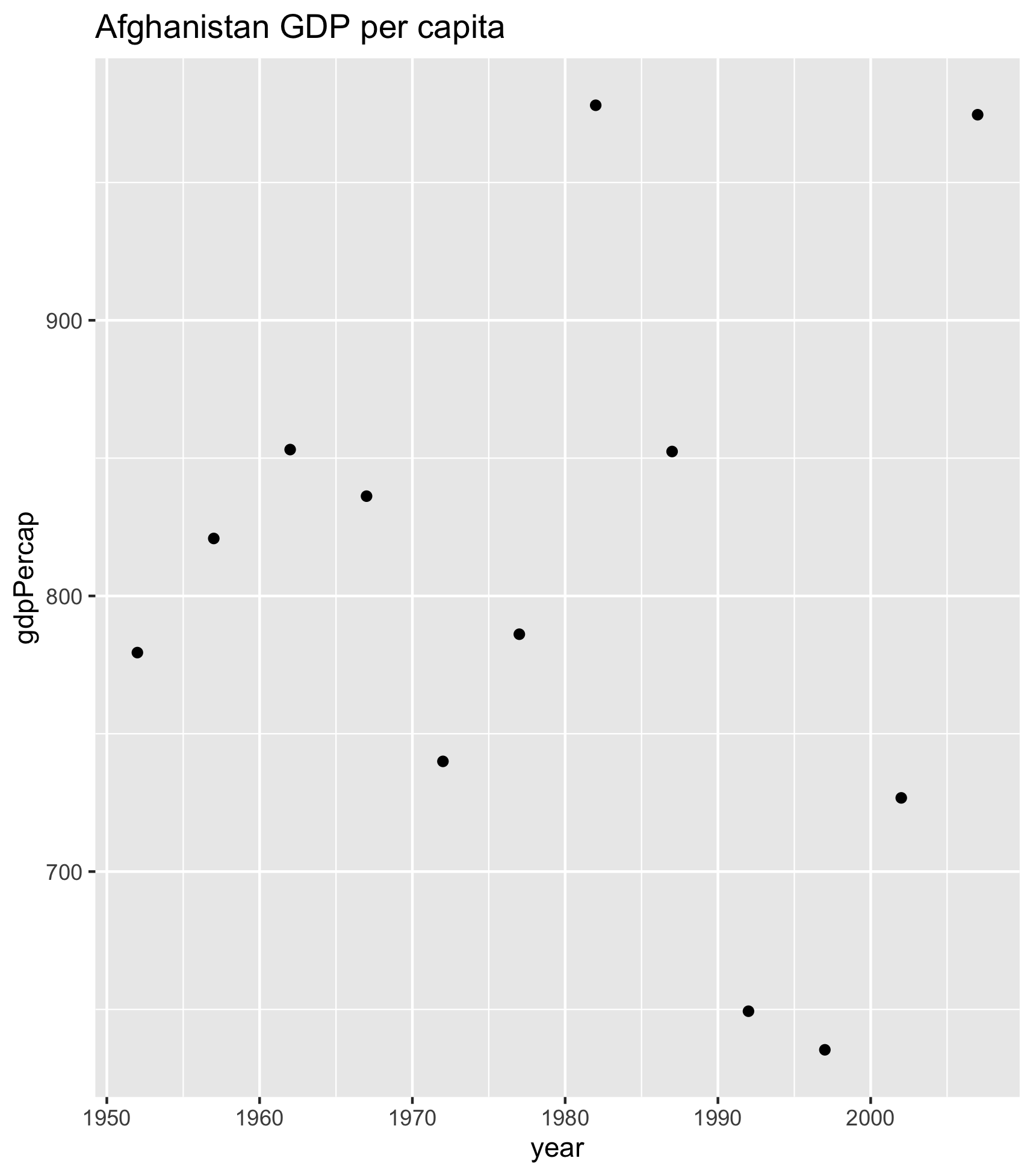
Let’s start off with what this would look like for just one country. I’m going to demonstrate with Afghanistan:
## filter the country to plot
gap_to_plot <- gapminder %>%
  filter(country == "Afghanistan")

## plot
my_plot <- ggplot(data = gap_to_plot, aes(x = year, y = gdp_per_cap)) +
  geom_point() +
  labs(title = "Afghanistan")
Let’s actually give this a better title than just the country name.
Let’s use the function str_c() to paste two strings
together so that the title is more descriptive. Use ?str_c
to see what the “sep” variable does.
## filter the country to plot
gap_to_plot <- gapminder %>%
  filter(country == "Afghanistan")

## plot
my_plot <- ggplot(data = gap_to_plot, aes(x = year, y = gdp_per_cap)) +
  geom_point() +
  ## add title and save
  labs(title = str_c("Afghanistan", "GDP per capita", sep = " "))
And as a last step, let’s save this figure.
## filter the country to plot
gap_to_plot <- gapminder %>%
  filter(country == "Afghanistan")

## plot
my_plot <- ggplot(data = gap_to_plot, aes(x = year, y = gdp_per_cap)) +
  geom_point() +
  ## add title and save
  labs(title = str_c("Afghanistan", "GDP per capita", sep = " "))

ggsave(filename = "Afghanistan_gdp_per_cap.png", plot = my_plot)
OK. So we can check our repo in the file pane (bottom right of RStudio) and see the generated figure:
Thinking ahead: cleaning up our code
Now, in our code above, we’ve had to write out “Afghanistan” several times. This makes it not only typo-prone as we type it each time, but if we wanted to plot another country, we’d have to write that in 3 places too. It is not setting us up for an easy time in our future, and thinking ahead in programming is something to keep in mind.
Instead of having “Afghanistan” written 3 times, let’s instead create an object that we will assign “Afghanistan” to. We won’t name our object “country” because that’s a column header with gapminder, and will just confuse us. Let’s make it distinctive: let’s write cntry (country without vowels):
## create country variable
cntry <- "Afghanistan"
Now, we can replace each "Afghanistan" with our variable
cntry. We will have to introduce a str_c()
statement in the ggsave() function too, and we want to
separate by nothing ("") because we don’t want spaces in
our filenames.
## create country variable
cntry <- "Afghanistan"

## filter the country to plot
gap_to_plot <- gapminder %>%
  filter(country == cntry)

## plot
my_plot <- ggplot(data = gap_to_plot, aes(x = year, y = gdp_per_cap)) +
  geom_point() +
  ## add title and save
  labs(title = str_c(cntry, "GDP per capita", sep = " "))
## note: there are many ways to create filenames with str_c(), str_c() or file.path(); we are doing this way for a reason.

ggsave(filename = str_c(cntry, "_gdp_per_cap.png", sep = ""), plot = my_plot)
Let’s run this. Great! it saved our figure (I can tell this because the timestamp in the Files pane has updated!)
for loop basic structure
Now, how about if we want to plot not only Afghanistan, but other
countries as well? There wasn’t actually that much code needed to get us
here, but we definitely do not want to copy this for every country. Even
if we copy-pasted and switched out the country assigned to the
cntry variable, it would be very typo-prone. Plus, what if
you wanted to instead plot life_exp? You’d have to remember to change it
each time… it quickly gets messy.
Better with a for loop. This will let us cycle through
and do what we want to each thing in turn. If you want to iterate over a
set of values, and perform the same operation on each, a
for loop will do the job.
Sit back and watch me for a few minutes while we develop the
for loop. Then we’ll give you time to do this on
your computers as well.
The basic structure of a for loop is:
for (each_item in set_of_items) {
  do a thing
}
Note the ( ) and the { }. We talk about
iterating through each item in the for loop, which makes
each item an iterator.
So looking back at our Afghanistan code: all of this is pretty much the “do a thing” part. And we can see that there are only a few places that are specific to Afghanistan. If we could make those places not specific to Afghanistan, we would be set.
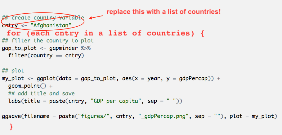
Let’s paste from what we had before, and modify it. I’m also going to
use RStudio’s indentation help to indent the lines within the
for loop by highlighting the code in this chunk and going
to Code > Reindent Lines (shortcut: command I)
## create country variable
cntry <- "Afghanistan"
for (each cntry in a list_of_countries) {

  ## filter the country to plot
  gap_to_plot <- gapminder %>%
    filter(country == cntry)

  ## plot
  my_plot <- ggplot(data = gap_to_plot, aes(x = year, y = gdp_per_cap)) +
    geom_point() +
    ## add title and save
    labs(title = str_c(cntry, "GDP per capita", sep = " "))

  ggsave(filename = str_c(cntry, "_gdp_per_cap.png", sep = ""), plot = my_plot)

}
Executable for loop!
OK. So let’s start with the beginning of the for loop.
We want a list of countries that we will iterate through. We can do that
by adding this code before the for loop.
## create a list of countries
country_list <- c("Albania", "Canada", "Spain")

for (cntry in country_list) {

  ## filter the country to plot
  gap_to_plot <- gapminder %>%
    filter(country == cntry)

  ## plot
  my_plot <- ggplot(data = gap_to_plot, aes(x = year, y = gdp_per_cap)) +
    geom_point() +
    ## add title and save
    labs(title = str_c(cntry, "GDP per capita", sep = " "))

  ggsave(filename = str_c(cntry, "_gdp_per_cap.png", sep = ""), plot = my_plot)
}
At this point, we do have a functioning for loop. For
each item in the country_list, the for loop
will iterate over the code within the { }, changing
cntry each time as it goes through the list. And we can see
it works because we can see them appear in the files pane at the bottom
right of RStudio!
Great! And it doesn’t matter if we just use these three countries or all the countries–let’s try it.
But first let’s create a figure directory and make sure it saves there since it’s going to get out of hand quickly. We could do this from the Finder/Windows Explorer, or from the “Files” pane in RStudio by clicking “New Folder” (green plus button). But we are going to do it in R. A folder is called a directory:
dir.create("figures")

## create a list of countries
country_list <- unique(gapminder$country) # ?unique() returns the unique values

for (cntry in country_list) {

  ## filter the country to plot
  gap_to_plot <- gapminder %>%
    filter(country == cntry)

  ## plot
  my_plot <- ggplot(data = gap_to_plot, aes(x = year, y = gdp_per_cap)) +
    geom_point() +
    ## add title and save
    labs(title = str_c(cntry, "GDP per capita", sep = " "))

  ## add the figures/ folder
  ggsave(filename = str_c("figures/", cntry, "_gdp_per_cap.png", sep = ""), plot = my_plot)
}
So that took a little longer than just the 3, but still super fast.
for loops are sometimes just the thing you need to iterate
over many things in your analyses.
Clean up our repo
OK we now have 142 figures that we just created. They exist locally on our computer, and we have the code to recreate them anytime. But, we don’t really need to push them to GitHub. Let’s delete the figures/ folder and see it disappear from the Git tab. An alternative to deleting the figures would be to add them to our .gitignore file. Read more about that here and play around with it.
Your turn
Use the worksheet we copied from the cloned GitHub repo to
- Modify our
forloop so that it:- loops through countries in Europe only
- plots the product of gdp_per_cap and population size per year (should approximate the total GDP) instead of the gdp_per_cap
- saves the plots to a new subfolder inside the (recreated) figures folder called “Europe”.
- Sync to GitHub
Answer
click to see our approach
dir.create("figures")
dir.create("figures/Europe")

## create a list of countries. Calculations go here, not in the for loop
gap_europe <- gapminder %>%
  filter(continent == "Europe") %>%
  mutate(gdp_tot = gdp_per_cap * pop)

country_list <- unique(gap_europe$country) # ?unique() returns the unique values

for (cntry in country_list) { # (cntry = country_list[1])

  ## filter the country to plot
  gap_to_plot <- gap_europe %>%
    filter(country == cntry)

  ## add a print message to see what's plotting
  print(str_c("Plotting", cntry))

  ## plot
  my_plot <- ggplot(data = gap_to_plot, aes(x = year, y = gdp_tot)) +
    geom_point() +
    ## add title and save
    labs(title = str_c(cntry, "GDP", sep = " "))

  ggsave(filename = str_c("figures/Europe/", cntry, "_gdp_tot.png", sep = ""), plot = my_plot)
}
Notice how we put the calculation of gdp_per_cap *
pop outside the for loop. It could have gone
inside, but it’s an operation that could be done just one time before
hand (outside the loop) rather than multiple times as you go (inside the
for loop).
Conditional statements with if and
else
Often when we’re coding we want to control the flow of our actions. This can be done by setting actions to occur only if a condition or a set of conditions are met.
In R and other languages, these are called “if statements”.
if statement basic structure
# if
if (condition is true) {
  do something
}

# if, else
if (condition is true) {
  do something
} else {  # that is, if the condition is false,
  do something different
}
Let’s bring this concept into our for loop for Europe
that we’ve just created. What if we want to add the label “Estimated” to
countries for which the values were estimated rather than based on
official reported statistics? Here’s what we’d do.
First, import csv file with information on whether data was estimated or reported, and join to gapminder dataset:
est <- read_csv('https://raw.githubusercontent.com/OHI-Science/data-science-training/master/data/countries_estimated.csv')
gapminder_est <- left_join(gapminder, est)
dir.create("figures")
dir.create("figures/Europe")
## create a list of countries. Calculations go here, not in the for loop
gap_europe <- gapminder_est %>% # Here we use the gapminder_est that includes information on whether data were estimated
filter(continent == "Europe") %>%
mutate(gdp_tot = gdp_per_cap * pop)
country_list <- unique(gap_europe$country) # ?unique() returns the unique values
for (cntry in country_list) { # (cntry = country_list[1])
## filter the country to plot
gap_to_plot <- gap_europe %>%
filter(country == cntry)
## add a print message to see what's plotting
print(str_c("Plotting", cntry))
## plot
my_plot <- ggplot(data = gap_to_plot, aes(x = year, y = gdp_tot)) +
geom_point() +
## add title and save
labs(title = str_c(cntry, "GDP", sep = " "))
## if estimated, add that as a subtitle.
if (gap_to_plot$estimated == "yes") {
## add a print statement just to check
print(str_c(cntry, " data are estimated"))
my_plot <- my_plot +
labs(subtitle = "Estimated data")
}
# Warning message:
# In if (gap_to_plot$estimated == "yes") { :
# the condition has length > 1 and only the first element will be used
ggsave(filename = str_c("figures/Europe/", cntry, "_gdp_tot.png", sep = ""),
plot = my_plot)
} This worked, but we got a warning message with the if
statement. This is because if we look at
gap_to_plot$estimated, it is many “yes”s or “no”s, and the
if statement works just on the first one. We know that if any are yes,
all are yes, but you can imagine that this could lead to problems down
the line if you didn’t know that. So let’s be explicit:
Executable if statement
dir.create("figures")
dir.create("figures/Europe")

## create a list of countries. Calculations go here, not in the for loop
gap_europe <- gapminder_est %>%  # Here we use the gapminder_est that includes information on whether data were estimated
  filter(continent == "Europe") %>%
  mutate(gdp_tot = gdp_per_cap * pop)

country_list <- unique(gap_europe$country) # ?unique() returns the unique values

for (cntry in country_list) { # (cntry = country_list[1])

  ## filter the country to plot
  gap_to_plot <- gap_europe %>%
    filter(country == cntry)

  ## add a print message to see what's plotting
  print(str_c("Plotting", cntry))

  ## plot
  my_plot <- ggplot(data = gap_to_plot, aes(x = year, y = gdp_tot)) +
    geom_point() +
    ## add title and save
    labs(title = str_c(cntry, "GDP", sep = " "))

## if estimated, add that as a subtitle.
if (any(gap_to_plot$estimated == "yes")) { # any() will return a single TRUE or FALSE

    ## add a print statement just to check
    print(str_c(cntry, " data are estimated"))

    my_plot <- my_plot +
      labs(subtitle = "Estimated data")
  }

  ggsave(filename = str_c("figures/Europe/", cntry, "_gdp_tot.png", sep = ""),
         plot = my_plot)

}
OK so this is working as we expect! Note that we do not need an
else statement above, because we only want to do something
(add a subtitle) if one condition is met. But what if we want to add a
different subtitle based on another condition, say where the data are
reported, to be extra explicit about it?
Executable if/else statement
dir.create("figures")
dir.create("figures/Europe")

## create a list of countries. Calculations go here, not in the for loop
gap_europe <- gapminder_est %>%  # Here we use the gapminder_est that includes information on whether data were estimated
  filter(continent == "Europe") %>%
  mutate(gdp_tot = gdp_per_cap * pop)

country_list <- unique(gap_europe$country) # ?unique() returns the unique values

for (cntry in country_list) { # (cntry = country_list[1])

  ## filter the country to plot
  gap_to_plot <- gap_europe %>%
    filter(country == cntry)

  ## add a print message to see what's plotting
  print(str_c("Plotting", cntry))

  ## plot
  my_plot <- ggplot(data = gap_to_plot, aes(x = year, y = gdp_tot)) +
    geom_point() +
    ## add title and save
    labs(title = str_c(cntry, "GDP", sep = " "))

## if estimated, add that as a subtitle.
if (any(gap_to_plot$estimated == "yes")) { # any() will return a single TRUE or FALSE

    ## add a print statement just to check
    print(str_c(cntry, " data are estimated"))

    my_plot <- my_plot +
      labs(subtitle = "Estimated data")
} else {

  print(str_c(cntry, " data are reported"))

  my_plot <- my_plot +
    labs(subtitle = "Reported data") }

  ggsave(filename = str_c("figures/Europe/", cntry, "_gdp_tot.png", sep = ""),
         plot = my_plot)

}
Note that this works because we know there are only two conditions,
Estimated == yes and Estimated == no. In the
first if statement we asked for estimated data, and the
else condition gives us everything else (which we know is
reported). We can be explicit about setting these conditions in the
else clause by instead using an else if
statement. Below is how you would construct this in your
for loop, similar to above:
  if (any(gap_to_plot$estimated == "yes")) { # any() will return a single TRUE or FALSE

    print(str_c(cntry, "data are estimated"))

    my_plot <- my_plot +
      labs(subtitle = "Estimated data")
  } else if (any(gap_to_plot$estimated == "no")){

    print(str_c(cntry, "data are reported"))

    my_plot <- my_plot +
      labs(subtitle = "Reported data")

  }
This construction is necessary if you have more than two conditions to test for.
We can also add the conditional addition of the plot subtitle with
R’s ifelse() function. It works like this
ifelse(condition is true, perform action, perform alternative action)where the first argument is the condition or set of conditions to be
evaluated, the second argument is the action that is performed if the
condition is true, and the third argument is the action to be performed
if the condition is not true. We can add this directly within the
initial labs() layer of our plot for a more concise
expression that achieves the same goal:
dir.create("figures")
dir.create("figures/Europe")

## create a list of countries. Calculations go here, not in the for loop
gap_europe <- gapminder_est %>%  # Here we use the gapminder_est that includes information on whether data were estimated
  filter(continent == "Europe") %>%
  mutate(gdp_tot = gdp_per_cap * pop)

country_list <- unique(gap_europe$country) # ?unique() returns the unique values

for (cntry in country_list) { # (cntry = country_list[1])

  ## filter the country to plot
  gap_to_plot <- gap_europe %>%
    filter(country == cntry)

  ## add a print message to see what's plotting
  print(str_c("Plotting ", cntry))

  ## plot
  my_plot <- ggplot(data = gap_to_plot, aes(x = year, y = gdp_tot)) +
    geom_point() +
    ## add title and save
    labs(title = str_c(cntry, "GDP", sep = " "), subtitle = ifelse(any(gap_to_plot$estimated == "yes"), "Estimated data", "Reported data"))

  ggsave(filename = str_c("figures/Europe/", cntry, "_gdp_tot.png", sep = ""),
         plot = my_plot)

}
Exercises (if time allows)
Exercises from R for Data Science
Work with the specified datasets that are built into R or in the
listed packages. You can access them just by typing the name (for
flights you will have to first load the
nycflights13 package).
Write for loops to:
- Compute the mean of every column in
mtcars - Determine the type of each column in
nycflights13::flights - Compute the number of unique values in each column of
iris
Concluding remarks
for loops are typically slow compared to vector based
methods and frequently not the best available solution for implementing
iterations. We therefore recommend that you learn about other
approaches, especially the map functions and functional programming.
However, for loops are easy to implement and easy to
understand so in many cases they can be a good solution for simple
iterations.