Lesson 1: Introduction to R and RStudio
Overview
Welcome to the course. Please review the introductory slides describing the focus, content, and goal of this course.
We will not have time to provide a comprehensive introduction to R and RStudio. Today, we will focus on highlighting a few key functionalities and tips that will be important for this course and get us all on the same page. If you have not worked in R before, we strongly encourage you to work through a couple of the tutorials listed under “Other useful resources” below.
Acknowledgements and resources
Most of today’s lesson has been borrowed (with permission) from the Ocean Health Index Data Science Training
Other useful resources to check out include the following:
- Jenny Bryan’s STAT545 Chapter 2 R basics and workflows
- R Swirl interactive lessons
- Data Carpentry’s Introduction to R for Ecologists
RStudio has great resources about its IDE (IDE stands for integrated development environment):
Orientation: R and RStudio
In this course, we will be using R with RStudio. R is the base statistical computing environment. RStudio is an Interactive Development Environment (IDE) that makes it much easier to use R by helping us organize our work and do things like auto-complete, syntax highlighting etc.
After you install R and RStudio, you only need to open RStudio.
When you open RStudio, it will look like this:
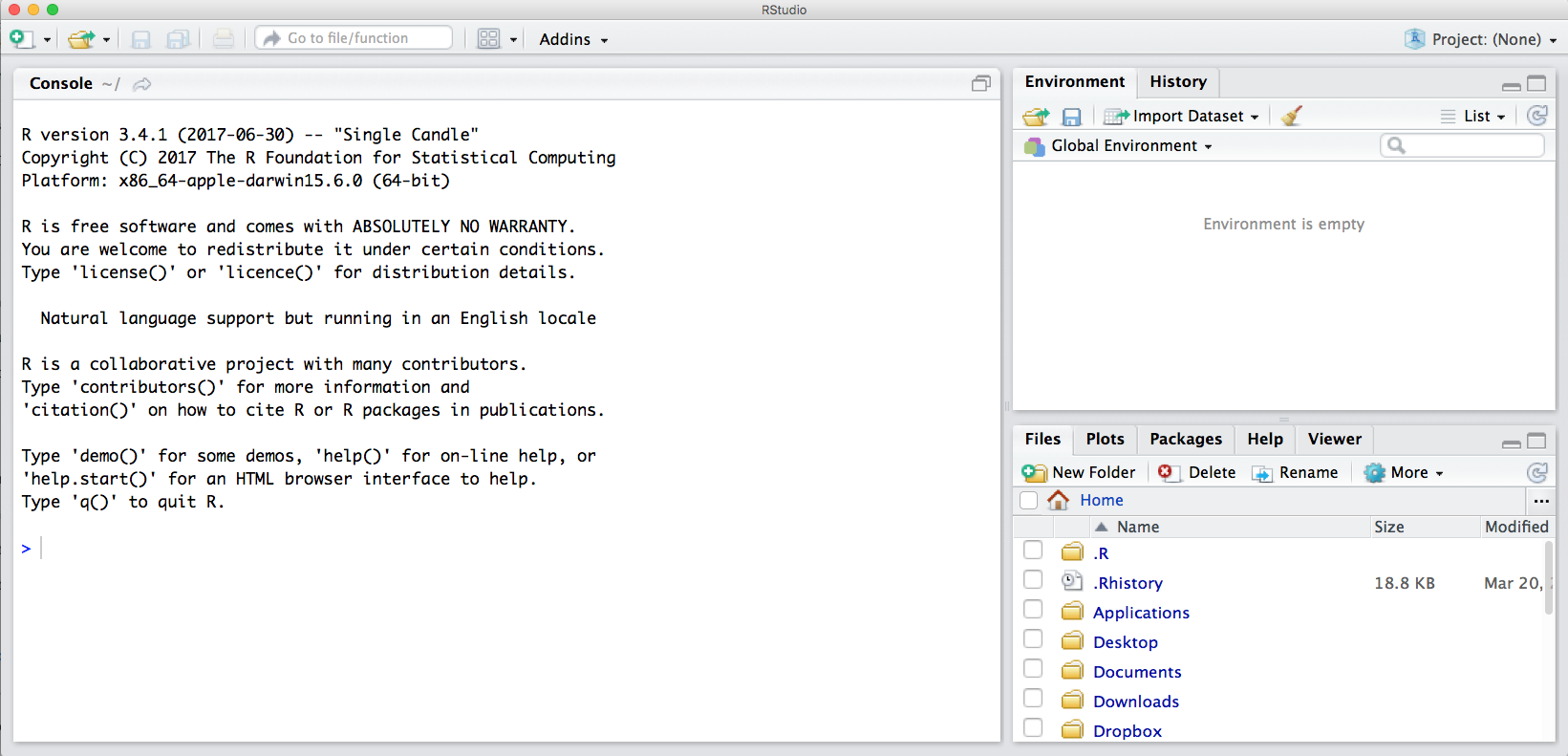
Notice the default panes:
- Console (entire left)
- Environment/History (tabbed in upper right)
- Files/Plots/Packages/Help (tabbed in lower right)
FYI: you can change the default location of the panes, among many other things: Customizing RStudio.
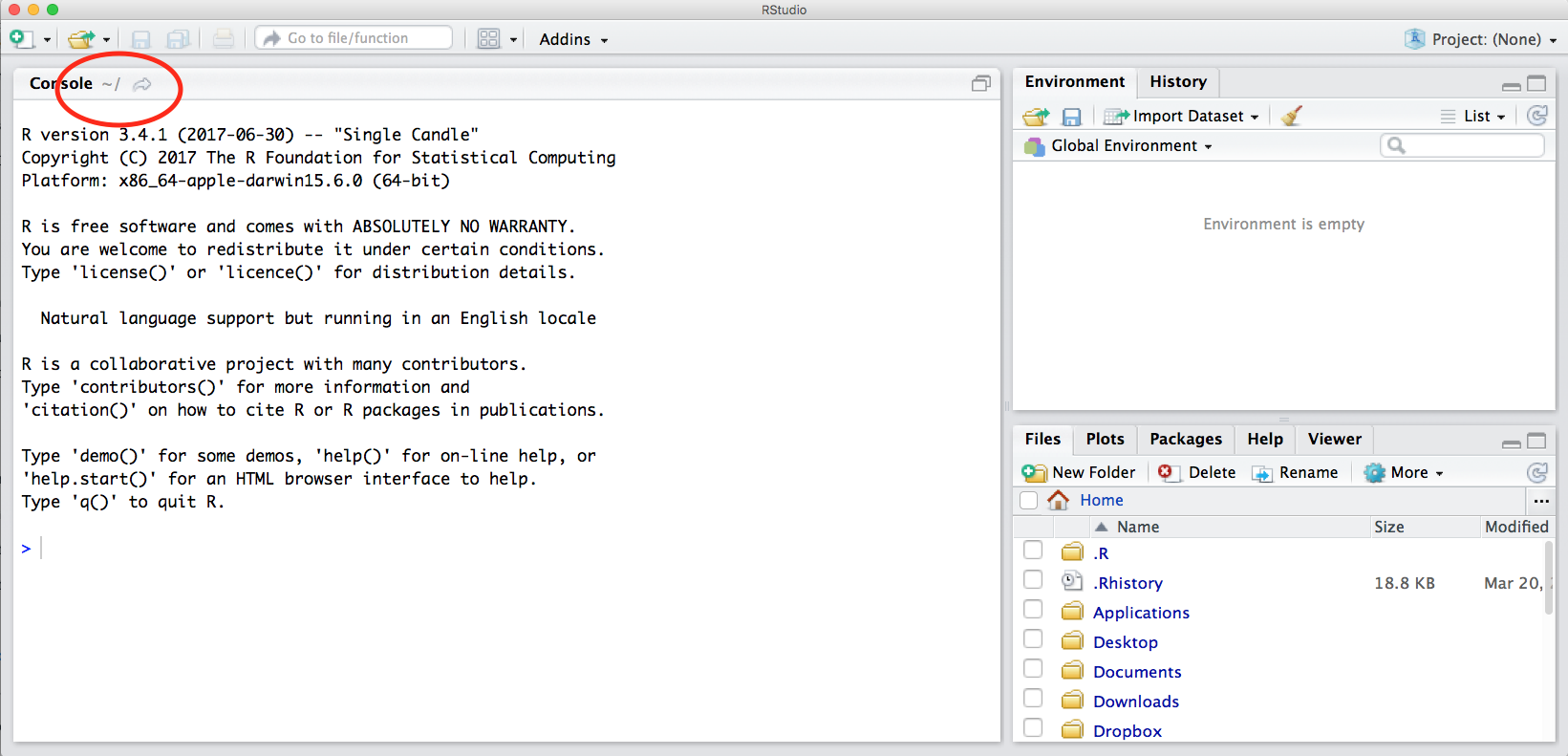
An important first question: where are we?
If you have opened RStudio for the first time, you’ll be in your Home
directory. This is noted by the ~/ at the top of the
console. You can see too that the Files pane in the lower right shows
what is in the Home directory where you are. You can navigate around
within that Files pane and explore, but note that you won’t change where
you are: even as you click through you’ll still be Home:
~/.
OK let’s go into the Console, where we interact with the live R process.
Make an assignment and then inspect the object you created by typing its name on its own.
x <- 3 * 4
x
## [1] 12In my head I hear, e.g., “x gets 12”.
All R statements where you create objects – “assignments” – have this
form: objectName <- value.
I’ll write it in the console with a hashtag #, which is
the way R comments so it won’t be evaluated.
## objectName <- value
## This is also how you write notes in your code to explain what you are doing.
Object names cannot start with a digit and cannot contain certain other characters such as a comma or a space. You will be wise to adopt a convention for demarcating words in names.
# i_use_snake_case
# other.people.use.periods
# evenOthersUseCamelCase
Shortcuts and autocomplete
Make an assignment
this_is_a_really_long_name <- 2.5To inspect this variable, instead of typing it, we can press the up arrow key and call your command history, with the most recent commands first. Let’s do that, and then delete the assignment:
this_is_a_really_long_name## [1] 2.5Another way to inspect this variable is to begin typing
this_…and RStudio will automatically have suggested
completions for you that you can select by hitting the tab key, then
press return.
Shortcuts You will make lots of assignments and the operator
<-is a pain to type. Don’t be lazy and use=, although it would work, because it will just sow confusion later. Instead, utilize RStudio’s keyboard shortcut: Alt + - (the minus sign). Notice that RStudio automagically surrounds<-with spaces, which demonstrates a useful code formatting practice. Code is miserable to read on a good day. Give your eyes a break and use spaces. RStudio offers many handy keyboard shortcuts. Also, Alt+Shift+K brings up a keyboard shortcut reference card. My most common shortcuts include command-Z (undo), and combinations of arrow keys in combination with shift/option/command (moving quickly up, down, sideways, with or without highlighting.
Error messages are your friends
Implicit contract with the computer / scripting language: Computer will do tedious computation for you. In return, you will be completely precise in your instructions. Typos matter. Case matters. Pay attention to how you type.
Remember that this is a language, not unsimilar to English! There are times you aren’t understood – it’s going to happen. There are different ways this can happen. Sometimes you’ll get an error. This is like someone saying ‘What?’ or ‘Pardon’? Error messages can also be more useful, like when they say ‘I didn’t understand what you said, I was expecting you to say blah’. That is a great type of error message. Error messages are your friend. Google them (copy-and-paste!) to figure out what they mean.
And also know that there are errors that can creep in more subtly, when you are giving information that is understood, but not in the way you meant. Like if I you are telling your European friend about a football game and she hears it but silently interprets it in a very different way (thinking football means soccer). This can leave you thinking you’ve gotten something across that the listener (or R) might silently interpret very differently. And as you continue telling your story the listener gets more and more confused… Clear communication is critical when you code: write clean, well documented code and check your work as you go to minimize these circumstances!
R functions, help pages
R has a mind-blowing collection of built-in functions that are used
with the same syntax: function name with parentheses around what the
function needs to do what it is supposed to do.
function_name(argument1 = value1, argument2 = value2, ...).
When you see this syntax, we say we are “calling the function”.
Let’s try using seq() which makes regular sequences of
numbers and, while we’re at it, demo more helpful features of
RStudio.
Type se and hit TAB. A pop up shows you possible
completions. Specify seq() by typing more to disambiguate
or using the up/down arrows to select. Notice the floating tool-tip-type
help that pops up, reminding you of a function’s arguments. If you want
even more help, press F1 as directed to get the full documentation in
the help tab of the lower right pane.
Type the arguments 1, 10 and hit return.
seq(1, 10)## [1] 1 2 3 4 5 6 7 8 9 10We could probably infer that the seq() function makes a
sequence, but let’s learn for sure. Type (and you can autocomplete) and
let’s explore the help page:
?seq
help(seq) # same as ?seq
The help page tells the name of the package in the top left, and broken down into sections:
- Description: An extended description of what the function does.
- Usage: The arguments of the function and their default values.
- Arguments: An explanation of the data each argument is expecting.
- Details: Any important details to be aware of.
- Value: The data the function returns.
- See Also: Any related functions you might find useful.
- Examples: Some examples for how to use the function.
seq(from = 1, to = 10) # same as seq(1, 10); R assumes by position## [1] 1 2 3 4 5 6 7 8 9 10seq(from = 1, to = 10, by = 2)## [1] 1 3 5 7 9The above also demonstrates something about how R resolves function
arguments. You can always specify in name = value form. But
if you do not, R attempts to resolve by position. So above, it is
assumed that we want a sequence from = 1 that goes
to = 10. Since we didn’t specify step size, the default
value of by in the function definition is used, which ends
up being 1 in this case. For functions I call often, I might use this
resolve by position for the first argument or maybe the first two. After
that, I always use name = value.
The examples from the help pages can be copy-pasted into the console for you to understand what’s going on. Remember we were talking about expecting there to be a function for something you want to do? Let’s try it.
Your turn
Exercise: Talk to your neighbor(s) and look up the help file for a function that you know or expect to exist. Here are some ideas:
?getwd(),?plot(),min(),max(),?mean(),?log()). And there’s also help for when you only sort of remember the function name: double-question mark:
??install Not all functions have (or require) arguments:
date()## [1] "Tue Aug 26 09:50:34 2025"Packages
So far we’ve been using a couple functions from base R, such as
seq() and date(). But, one of the amazing
things about R is that a vast user community is always creating new
functions and packages that expand R’s capabilities. In R, the
fundamental unit of shareable code is the package. A package bundles
together code, data, documentation, and tests, and is easy to share with
others. They increase the power of R by improving existing base R
functionalities, or by adding new ones.
The traditional place to download packages is from CRAN, the Comprehensive R Archive Network, which is where you downloaded R. You can also install packages from GitHub, which we’ll do tomorrow.
You don’t need to go to CRAN’s website to install packages, this can
be accomplished within R using the command
install.packages("package-name-in-quotes"). Let’s install a
small, fun package praise. You need to use quotes around
the package name.:
install.packages("praise")Now we’ve installed the package, but we need to tell R that we are
going to use the functions within the praise package. We do
this by using the function library().
What’s the difference between a package and a
library?
Sometimes there is a confusion between a package and a library, and you
can find people calling packages “libraries”.
Please don’t get confused: library() is the command used
to load a package, and it refers to the place where the package is
contained, usually a folder on your computer, while a package is the
collection of functions bundled conveniently.
library(praise)Now that we’ve loaded the praise package, we can use the
single function in the package, praise(), which returns a
randomized praise to make you feel better.
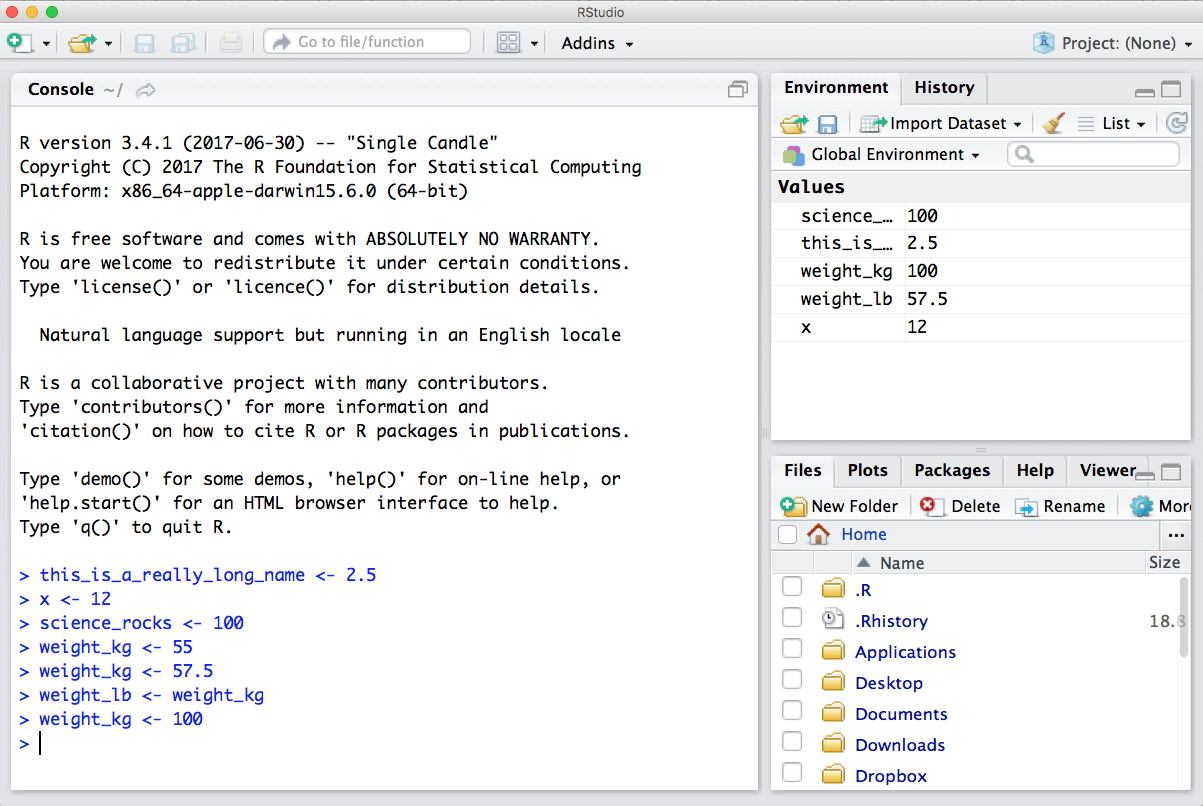
praise()## [1] "You are cat's meow!"Clearing the environment
Now look at the objects in your environment (workspace) – in the upper right pane. The workspace is where user-defined objects accumulate. If we try typing in the commands shown in the console below, we’ll see each of the objects we have created in our “Environment” pane.
You can also get a listing of these objects with a few different R commands:
objects()## [1] "this_is_a_really_long_name" "x"ls()## [1] "this_is_a_really_long_name" "x"If you want to remove the object named weight_kg, you
can do this:
rm(weight_kg)## Warning in rm(weight_kg): object 'weight_kg' not foundTo remove everything:
rm(list = ls())or click the broom in RStudio’s Environment pane.
But this command is problematic -see Jenny Bryan’s explanation.
For reproducibility, it is critical that you delete your objects and restart your R session frequently. You don’t want your whole analysis to only work in whatever way you’ve been working right now — you need it to work next week, after you upgrade your operating system, etc. Restarting your R session will help you identify and account for anything you need for your analysis.
We will keep coming back to this theme but let’s restart our R session together: Go to the top menus: Session > Restart R.
Your turn
Exercise: Clear your workspace, then create a few new variables. Create a variable that is the mean of a sequence of 1-20. What’s a good name for your variable? Does it matter what your ‘by’ argument is? Why?
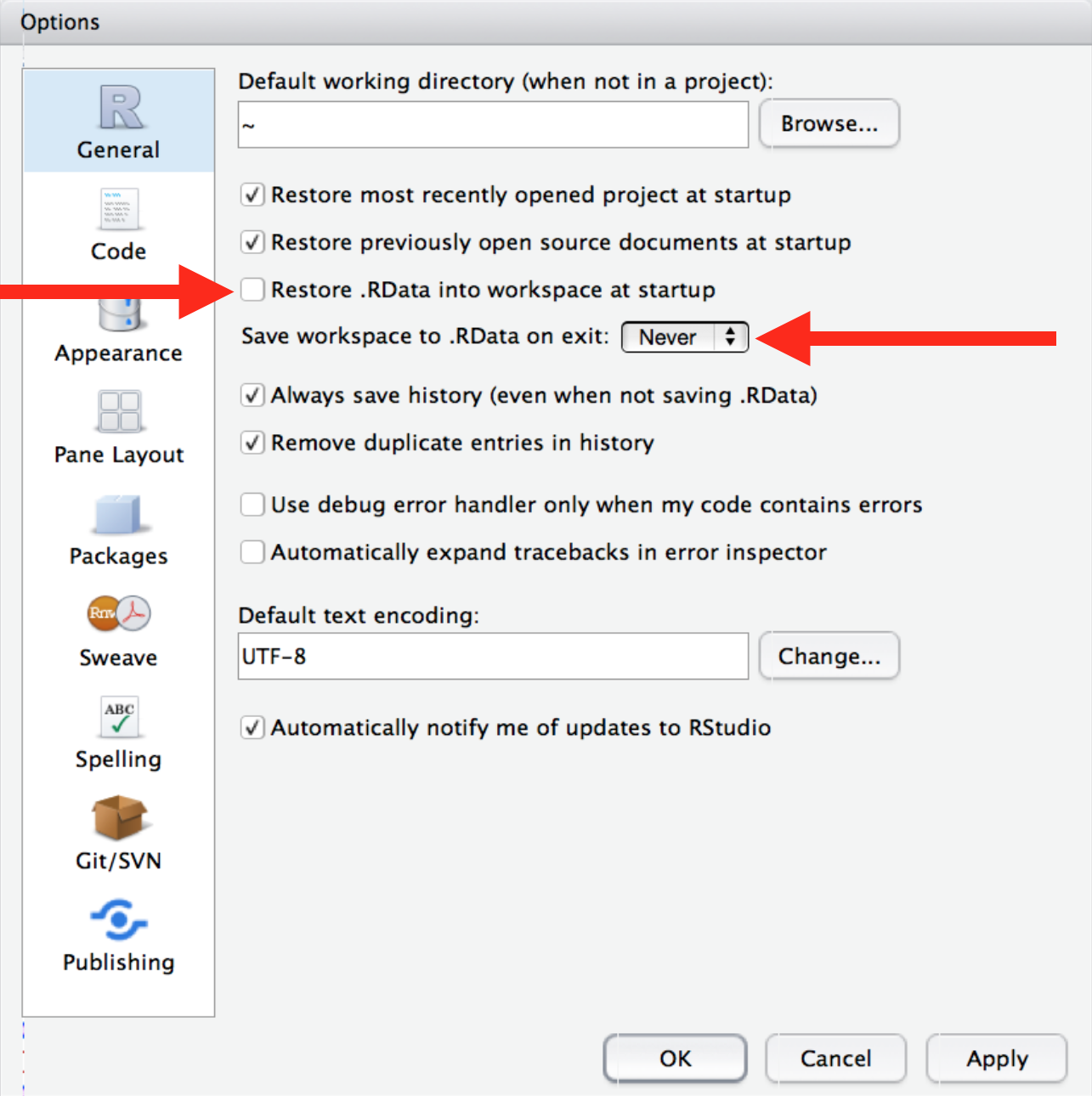
Highly recommended: Don’t save your workspace when you quit RStudio. Make this a default:
Go to “RStudio” -> “Preferences…” -> “General” (Or “Tools” -> “Options” -> “General” if you are on a Windows machine)
Uncheck “restore .RData into workspace on startup”
Select: “Save workspace to RData on exit:” Never
Home directory, relative vs. absolute paths and RStudio projects
See sections 8.2-8.4 in Grolemund and Wickham’s R for Data Science
Additional tips on RStudio projects here
During next class, we will set up an RStudio project for you to work in during this course (we’re waiting until next class because we want to integrate it with GitHub from the get-go).
Saving your code in scripts
See Chapter 6 in Grolemund and Wickham’s R for Data Science
If you’re new to R, this may all seem a little overwhelming right now. Don’t worry, we’ll keep coming back to revisit some of the key concepts outlined above as we work through the course.