Lesson 3: Version control and the Git/GitHub workflow
Readings
Other resources:
GitHub’s Get Started Documentation has a number of tutorials. “Hello World” is a good place to start
Happy Git with R by Jenny Bryan
GitHub for Project Management by Openscapes
Announcements
- The classroom is a little wide so it might be hard to see the screen
from the edges of the room. Please talk to us or write in the
feedbackchannel if you have suggestions for how we can make things work better in the room. - Homework 1 is due this Thursday at 10pm (submit through GitHub! – we’ll demo later).
- Auditors are welcome to submit homework assignments for useful practice and feedback.
- Jaime will host office hours Wednesday 10-11am in 311 Fernow Hall.
- Nina will host office hours 11.30-12am (right after class) this Thursday on the benches outside the classroom.
Learning objectives
By the end of this class you will be able to:
- Locate your personal GitHub repo through which you’ll be submitting homework and exercises for this course
- Create and edit plain text files on GitHub
- Navigate the commit history of a repository and a file on GitHub
- Clone a repo locally using RStudio
- Sync local changes to a file back to remote (and GitHub) with pull, stage, commit, push
- Describe the advantages of a project-oriented workflow in RStudio and set up a version-controlled project directory on your computer
Acknowledgements: Today’s lecture is adapted from the excellent R for Excel users course by Julia Stewart Lowndes and Allison Horst and the STAT457 course at UBC.
Introduction to Git and GitHub
Why should R users use GitHub?
Modern R users use GitHub because it helps make coding collaborative and social while also providing huge benefits to organization, archiving, and being able to find your files easily when you need them.
One of the most compelling reasons for me is that it ends (or nearly ends) the horror of keeping track of versions.
Basically, we get away from this:
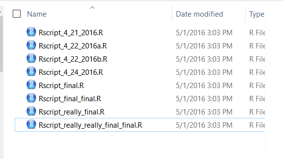
This is a nightmare not only because I have NO idea which is truly the version we used in that analysis we need to update, but because it is going to take a lot of detective work to see what actually changed between each file. Also, if we’re collaborating with other people on these documents and, for example, sharing them over email, it can become very tricky to ensure everyone always has the most current verion. Even if updates are always immediately shared, everyone’s bookkeeping can take a huge amount of time. Is everyone downloading an attachment, dragging it to wherever they organize this on their own computers, and then renaming everything? Hours and hours of all of our lives.
Fortunately there is Git and GitHub!
On GitHub, in this example you will likely only see a single file, which is the most recent version. GitHub’s job is to track who made any changes and when (so no need to save a copy with your name or date at the end), and it also requires that you write something human-readable that will be a breadcrumb for you in the future. It is also designed to be easy to compare versions, and you can easily revert to previous versions.
GitHub also supercharges you as a collaborator. First and foremost with Future You, but also sets you up to collaborate with Future Us!
GitHub, especially in combination with RStudio, is also game-changing for publishing and distributing. You can — and we will — publish and share files openly on the internet.
What is GitHub? And Git?
OK so what is GitHub? And Git?
Git is a program that you install on your computer: it is version control software that tracks changes to your files over time.
GitHub is an website that is essentially a social media platform for your Git-versioned files. GitHub stores all your versioned files as an archive, but also as allows you to interact with other people’s files and has management tools for the social side of software projects. It has many nice features to be able visualize differences between images, rendering & diffing map data files, render text data files, and track changes in text.
GitHub was developed for software development, so much of the functionality and terminology that is exciting for professional programmers (e.g., branches and pull requests) isn’t necessarily the right place for us as new R users to get started. We’ll get there soon, but for now, we will be learning and practicing GitHub’s features and terminology on a “need to know basis” as we start managing our projects with GitHub.
Account types
GitHub allows for cloud storage, like Google Drive and Dropbox do. But there’s a bit more structure than just storing files under your account:
- Repositories (aka “repos”): All files must be organized into repositories. Think of these as self-contained projects. These can either be public or private.
User Accounts vs. Organization Accounts (aka “Org”): All repositories belong to an account:
- A user account is the account you have made for yourself, and typically holds repositories related to your own work.
- An Organization account can be owned by multiple people, and
typically holds repositories relevant to a group (like
therkildsen-class).
Examples:
- The ggplot2 repo,
within its corresponding
tidyverseorganization - Our class
website within Nina’s user account
nt246
Say hello to your course repo on GitHub
In this course, you will not be working in repos in your own personal account because then we will not have edit access to your files. Instead, you will work within your personal course repo that we have created with a GitHub Classroom organization for the class. To access your personal course repo through which you will be submitting your assignments and communicating with us, click here. Select your name from the list (or just click continue if you don’t see your name there).
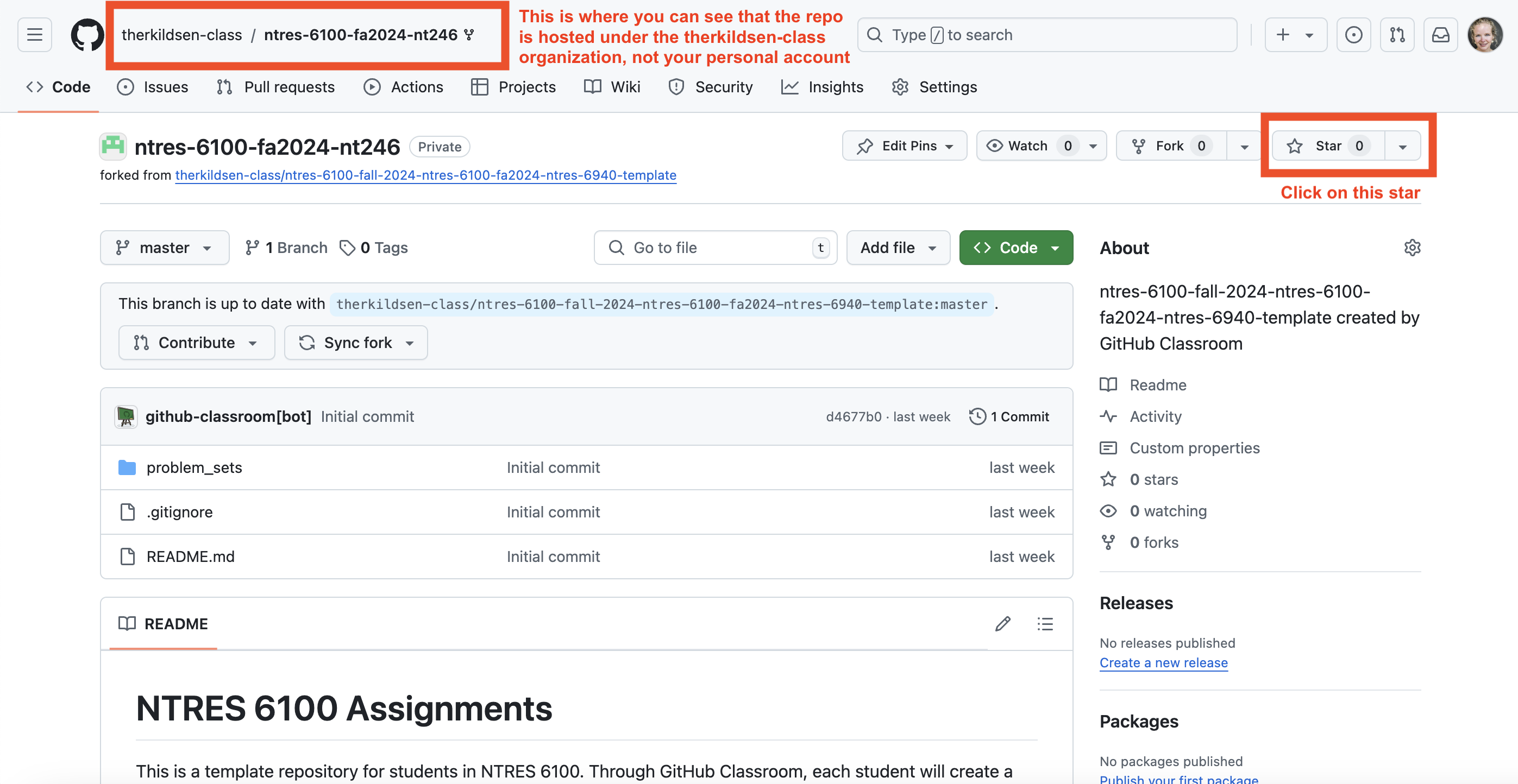
Once you land on your repo page, notice that it is hosted within our
course organizational account therkildsen-class, not your
personal account (see the path in the top left corner). To make this
repo also show up on your personal account page, click the “Star” button
on the top right of the page.
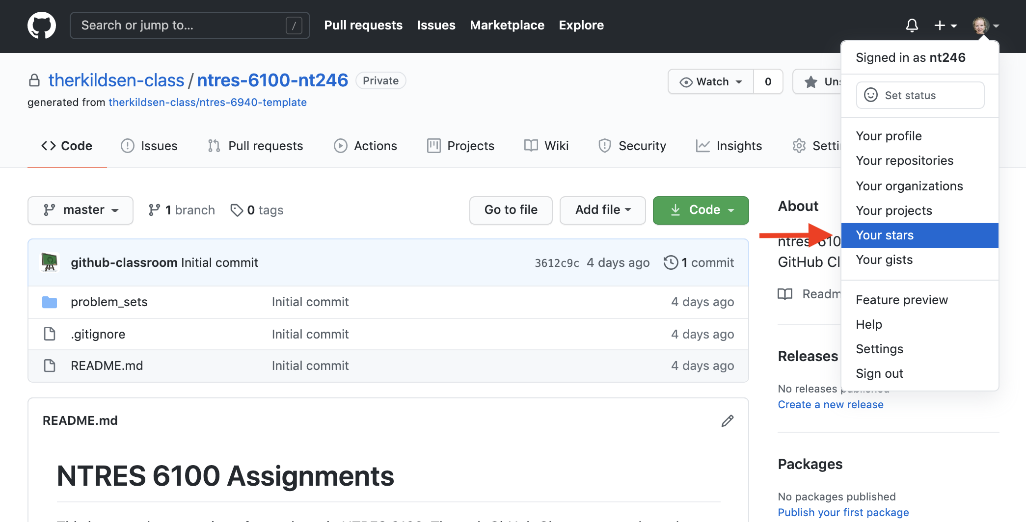
Now if you click on the profile information in the very top right
corner, and select the “Your stars” option, you’ll be taken to a list of
all the repos you have starred and your course repo should show up here
(it should be named something like
therkildsen-class/ntres-6100-assignments-YOUR_USER_NAME).
Click on the repo name to return to your course repo.
Interfacing with GitHub from our local computers using RStudio
We should all have set up Git on our local computers by now and have it connected to RStudio. If you don’t, follow the instructions here, and let us know if you run into problems.
Clone your repository using RStudio
We should all have identified our course repo on GitHub, i.e. in the cloud. Now, we will use RStudio to establish it locally on our computers: that is called “cloning”. Unlike downloading, cloning keeps all the version control and user information bundled with the files. Cloning is an important task when working with GitHub, so we’ll do it over and over again to establish the habit.
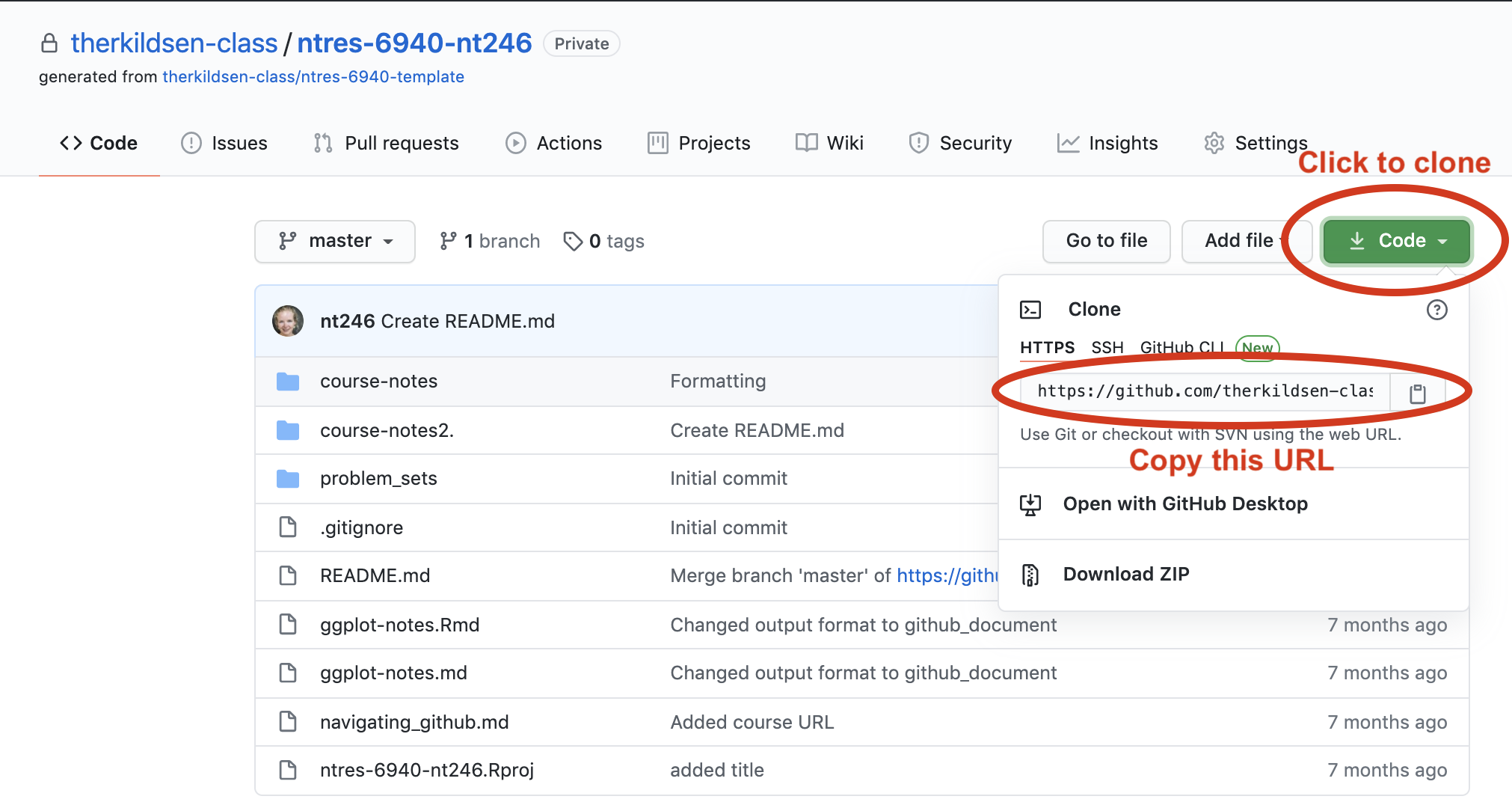
Copy the repo address
First, click the green “Code” button, then copy the web address of the repository you want to clone. We will use HTTPS.
Aside: HTTPS is default, and is method recommended by GitHub. You could alternatively set up with SSH, but we will not get into that here.
RStudio: New Project
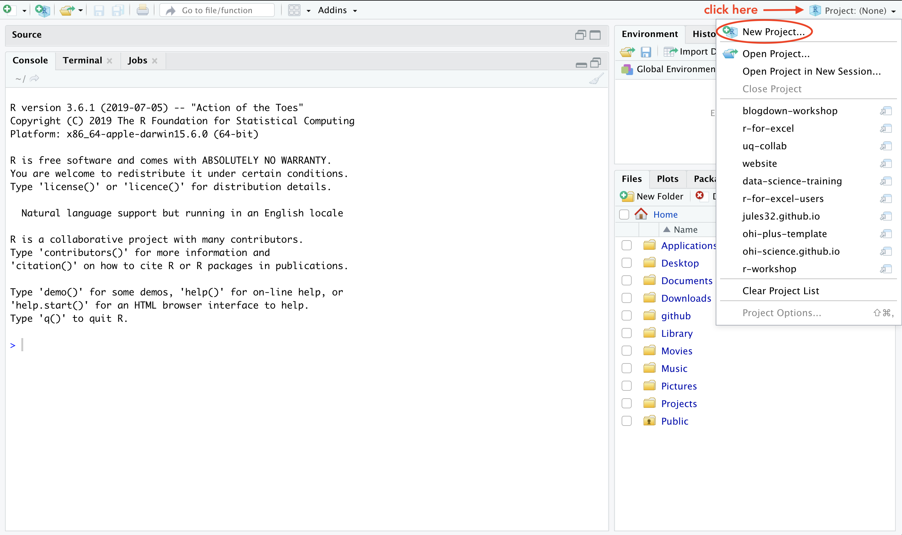
Now go to RStudio, and click on New Project. There are a few different ways; you could also go to File > New Project…, or click the little green + with the R box in the top left.
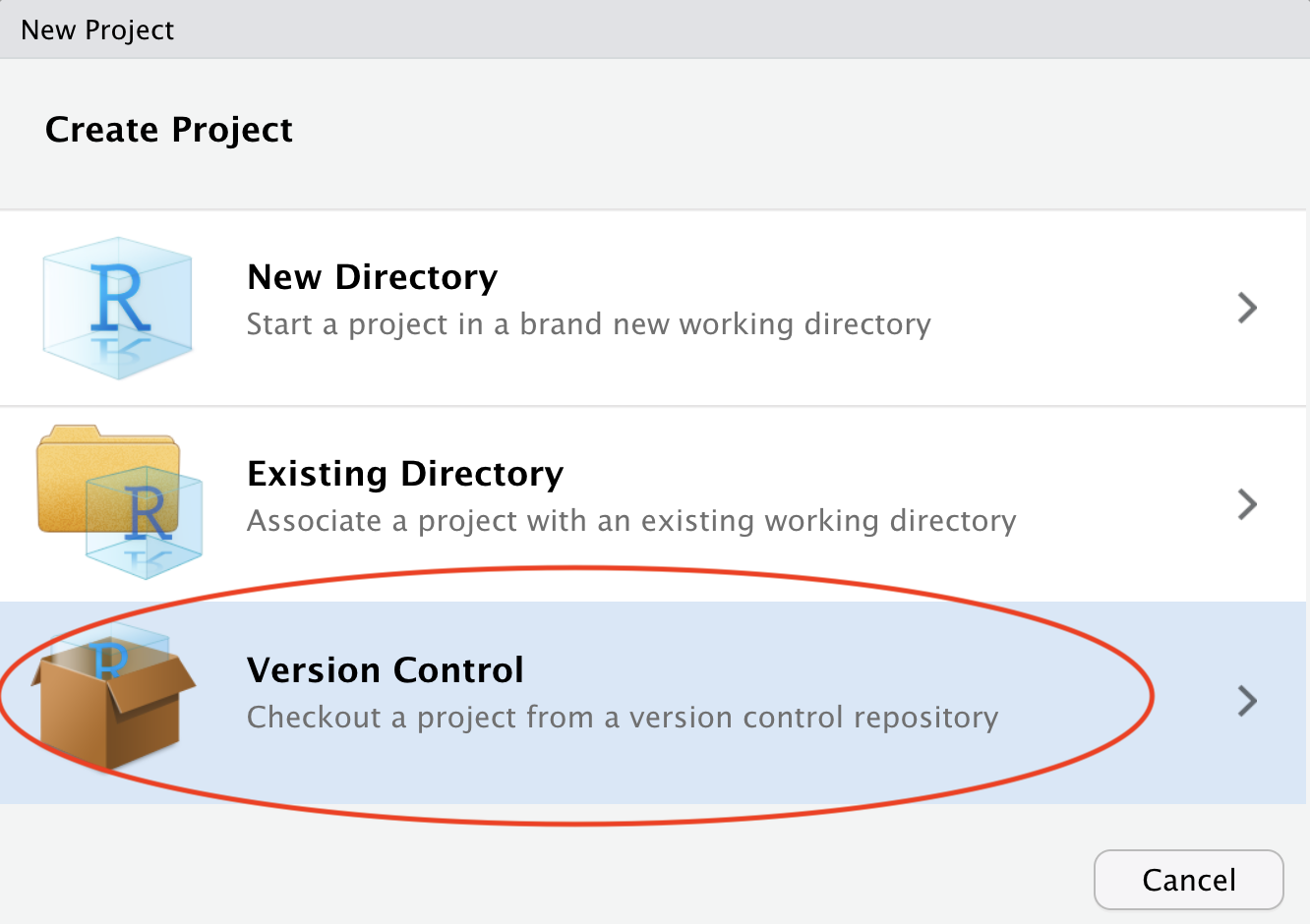
Select Version Control
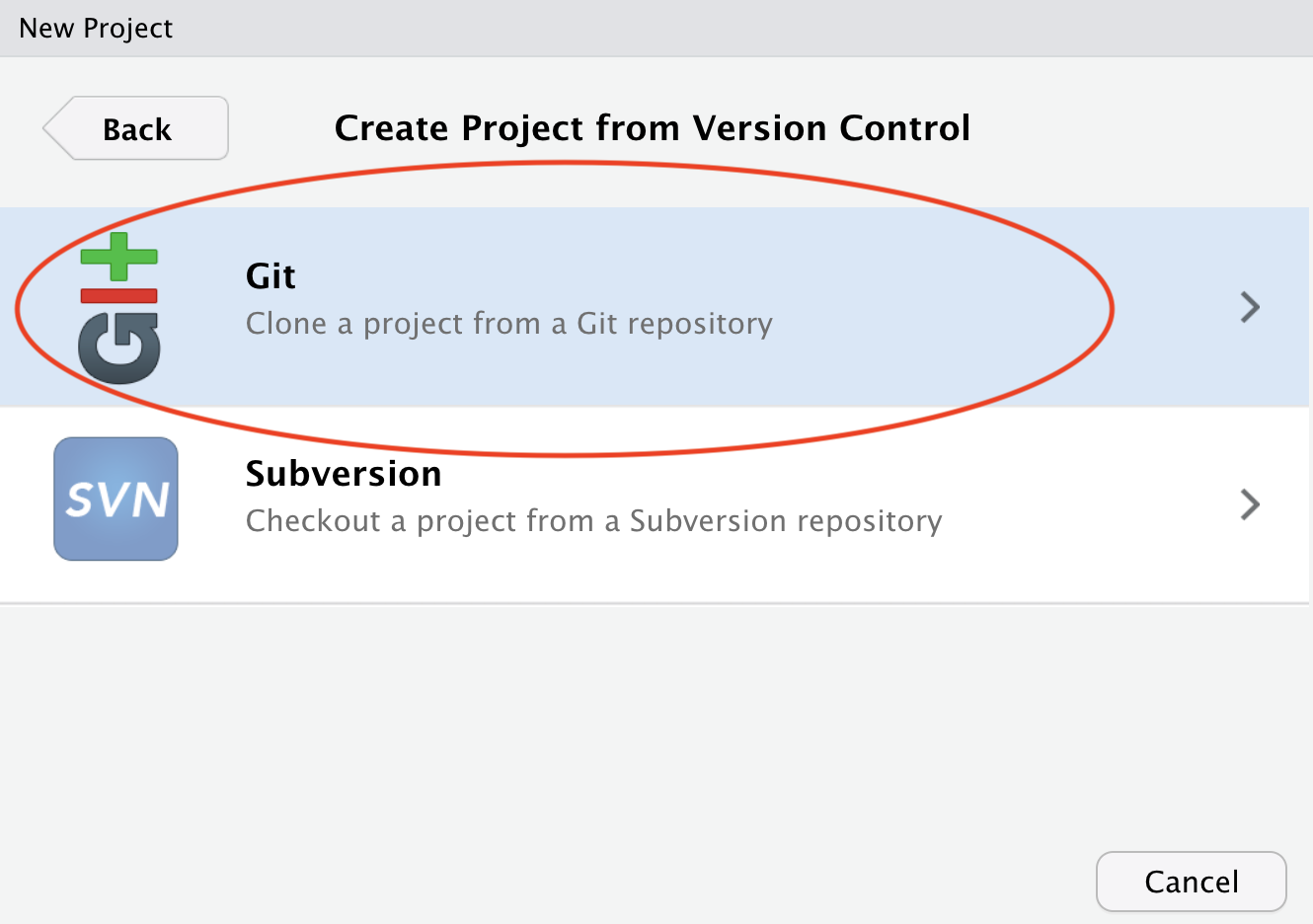
Select Git
Since we are using Git.
We got to this step during last class when we were confirming that our set-up has Git configured and connected to RStudio and GitHub correctly. Now, we will go ahead and actually clone our GitHub repo to our local computer.
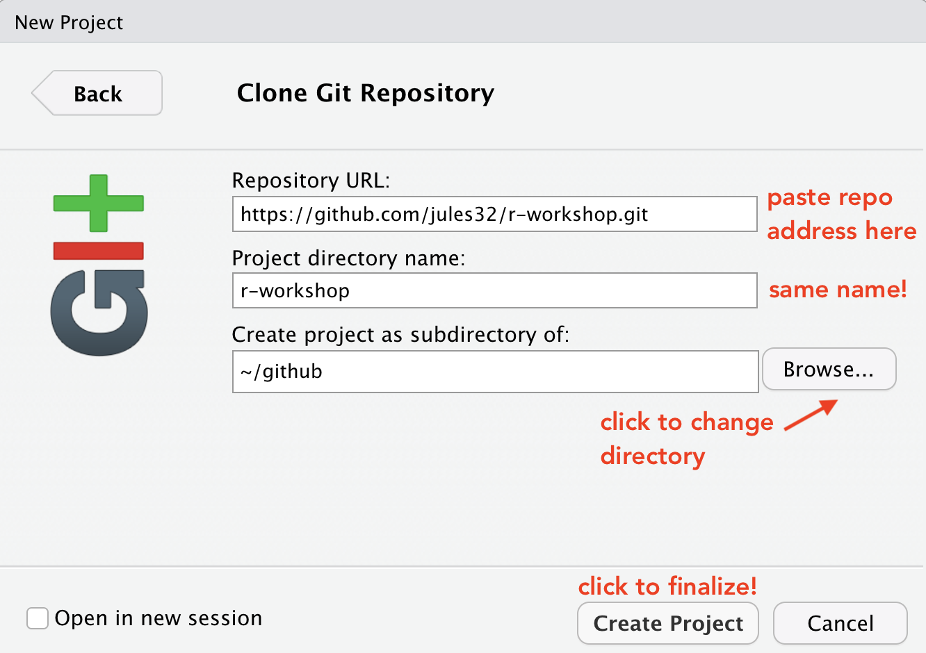
Paste the repo address
Paste the repo address (which is still in your clipboard) into in the “Repository URL” field. The “Project directory name” should auto-fill; if it does not press tab, or type it in. It is best practice to keep the “Project directory name” THE SAME as the repository name.
When cloned, this repository is going to become a folder on your computer.
At this point you can save this repo anywhere. Press “Browse…” to navigate to a folder and you have the option of creating a new folder.
There are different schools of thought but we think it is useful to
create a high-level folder where you will keep your GitHub repos to keep
them organized. We call ours github (all lowercase) and
keep it in our root folder (~/github), and so that is what
we will demonstrate here. We encourage you to do the same. Why? First of
all, you’ll always know where all your code is located, and it will
mirror the structure of what you see on GitHub. Second, it makes working
across users and machines easier if all your file paths start with
~/github/repo-name.
IMPORTANT: Make sure to not place it in folder tracked by a cloud storage service (e.g. DropBox, Google Drive or Box) because problems can arise when trying to sync folders with multiple systems.
Finally, click Create Project.
Admire and inspect your local repo
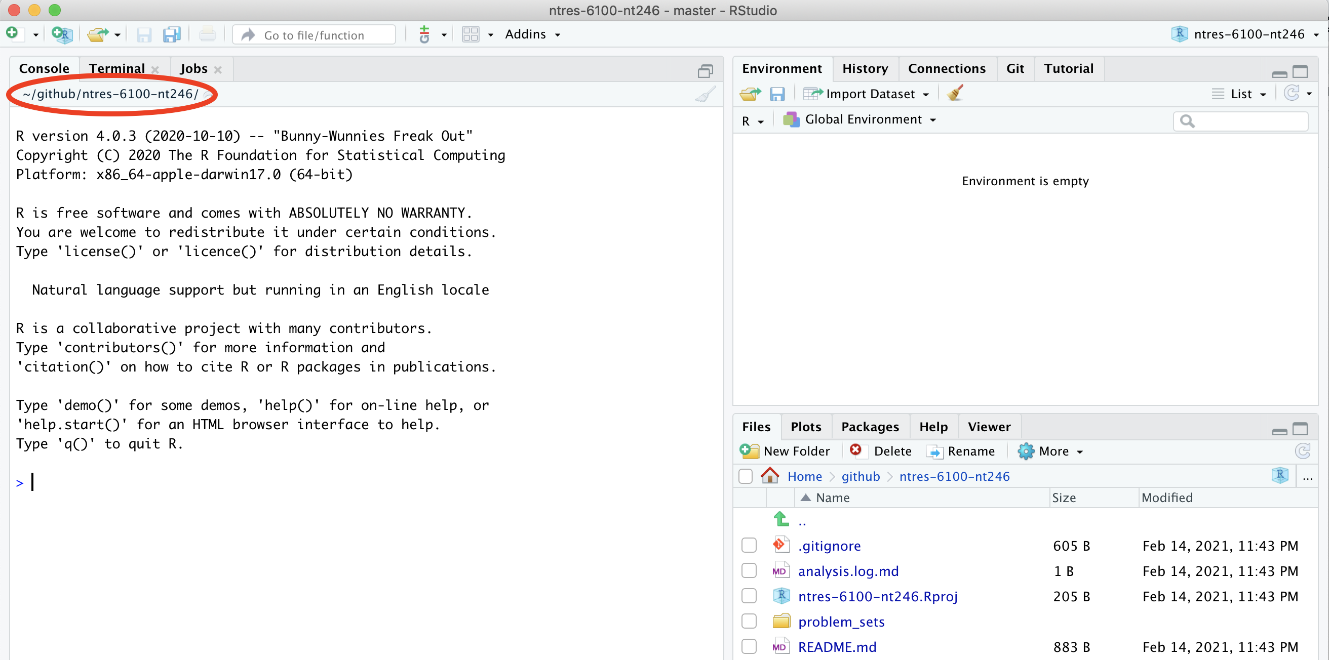
If everything went well, the repository will show up in RStudio!
The repository is also saved to the location you specified, and you can navigate to it as you normally would in Finder or Windows Explorer:
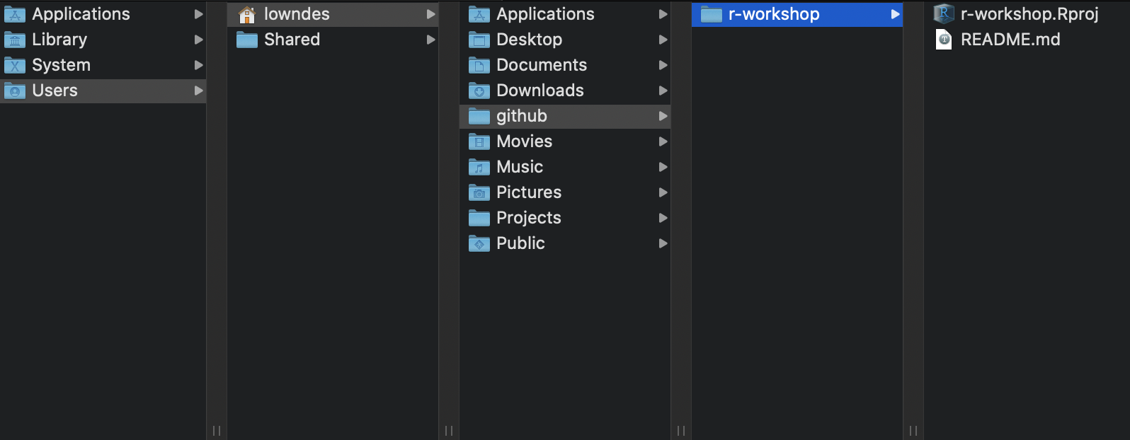
Hooray!
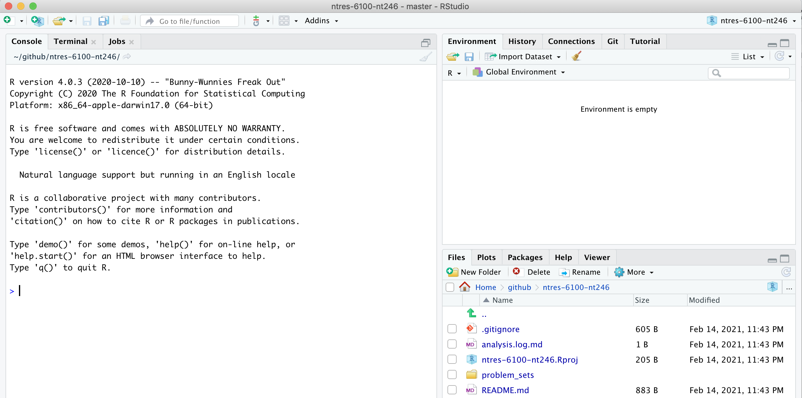
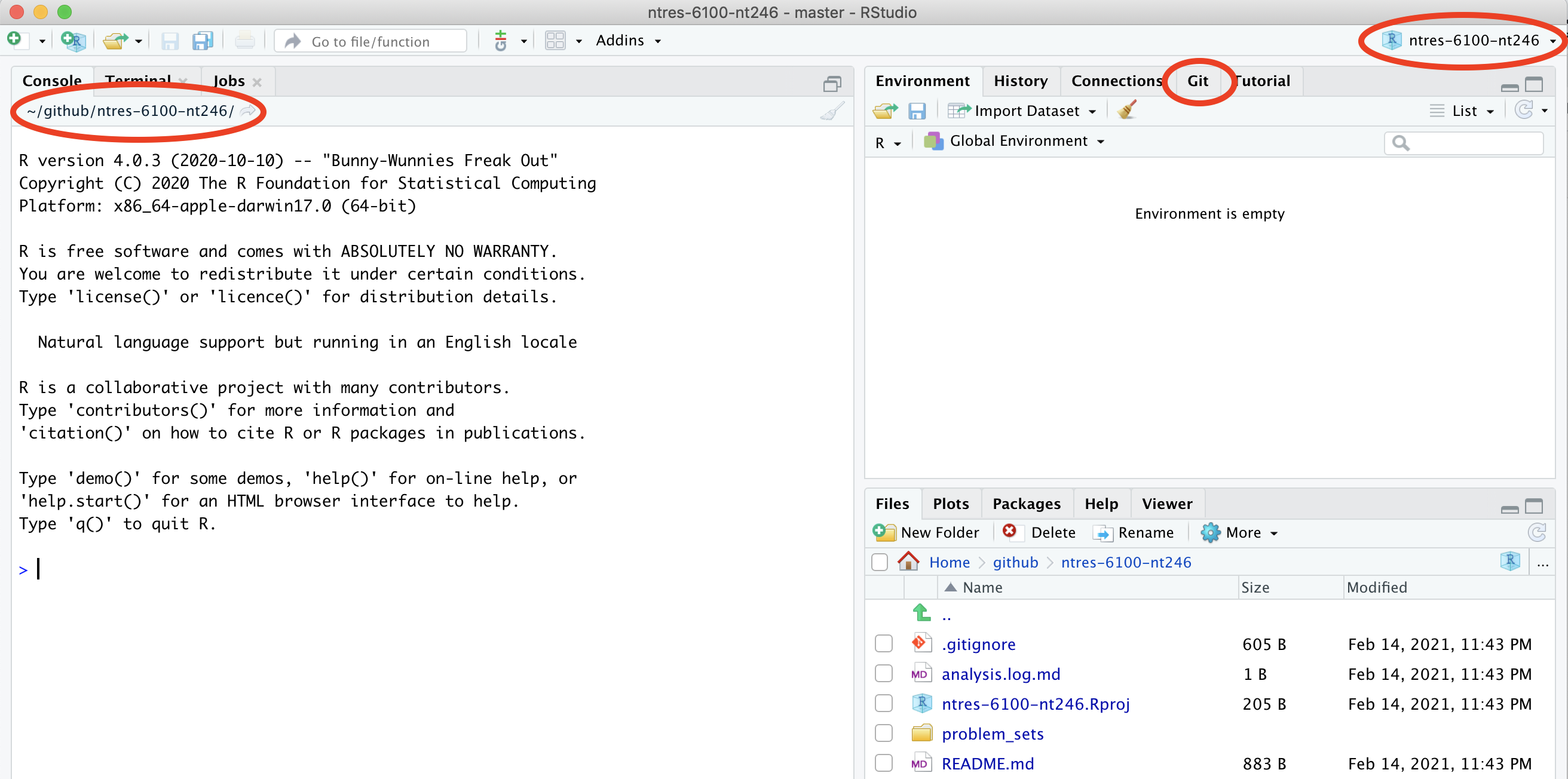
Let’s notice a few things:
First, our working directory is set to
~/github/ntres-6100-assignments-USERNAME, and
ntres-6100-assignments-USERNAME is also named in the top
right hand corner.
Second, we have a Git tab in the top right pane! Let’s click on it.
Our Git tab has 2 items:
- .gitignore file
- .Rproj file
These have been added to our repo by RStudio — we can also see them
in the File pane in the bottom right of RStudio. These are helper files
that RStudio has added to streamline our workflow with GitHub and R. We
will talk about these a bit more soon. One thing to note about these
files is that they begin with a period (.) which means they
are hidden files: they show up in the Files pane of RStudio but won’t
show up in your Finder or Windows Explorer.
Going back to the Git tab, both these files have little yellow icons
with question marks ?. This is GitHub’s way of saying: “I
am responsible for tracking everything that happens in this repo, but
I’m not sure what is going on with these files yet. Do you want me to
track them too?”
We will handle this in a moment; first let’s look at the README.md file.
Edit your README file
Let’s also open up the README.md. This is a Markdown
file, which is the same language we just learned with Quarto / R
Markdown. It’s like a Quarto file without the abilities to run code (but
we can see much of the formatting in the visual editor.
We will edit the file and illustrate how GitHub tracks files that have been modified (to complement seeing how it tracks files that have been added).
README files are common in programming; they are the first place that someone will look to see why code exists and how to run it.
In my README, I’ll edit the line that says:
Please indicate if you are **taking this class for credit** or **auditing**: and delete the option that does not apply to me.
When I save this, notice how it shows up in my Git tab. It has a blue “M”: GitHub is already tracking this file, and tracking it line-by-line, so it knows that something is different: it’s Modified with an M.
Great. Now let’s sync back to GitHub in 4 steps.
Sync from RStudio (local) to GitHub (remote)
Syncing to GitHub.com means 4 steps:
- Pull
- Stage
- Commit
- Push
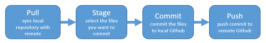
Pull
We start off by “Pulling” from the remote repository (github.com) to make sure that our local copy has the most up-to-date information that is available online. Right now, since we just created the repo and are the only ones that have permission to work on it, we can be pretty confident that there isn’t new information available. But we pull anyway because this is a very safe habit to get into for when you start collaborating with yourself across computers or others. Best practice is to pull often: it costs nothing (other than an internet connection).
Pull by clicking the teal Down Arrow. (Notice also how when you highlight a filename, a preview of the differences displays below).
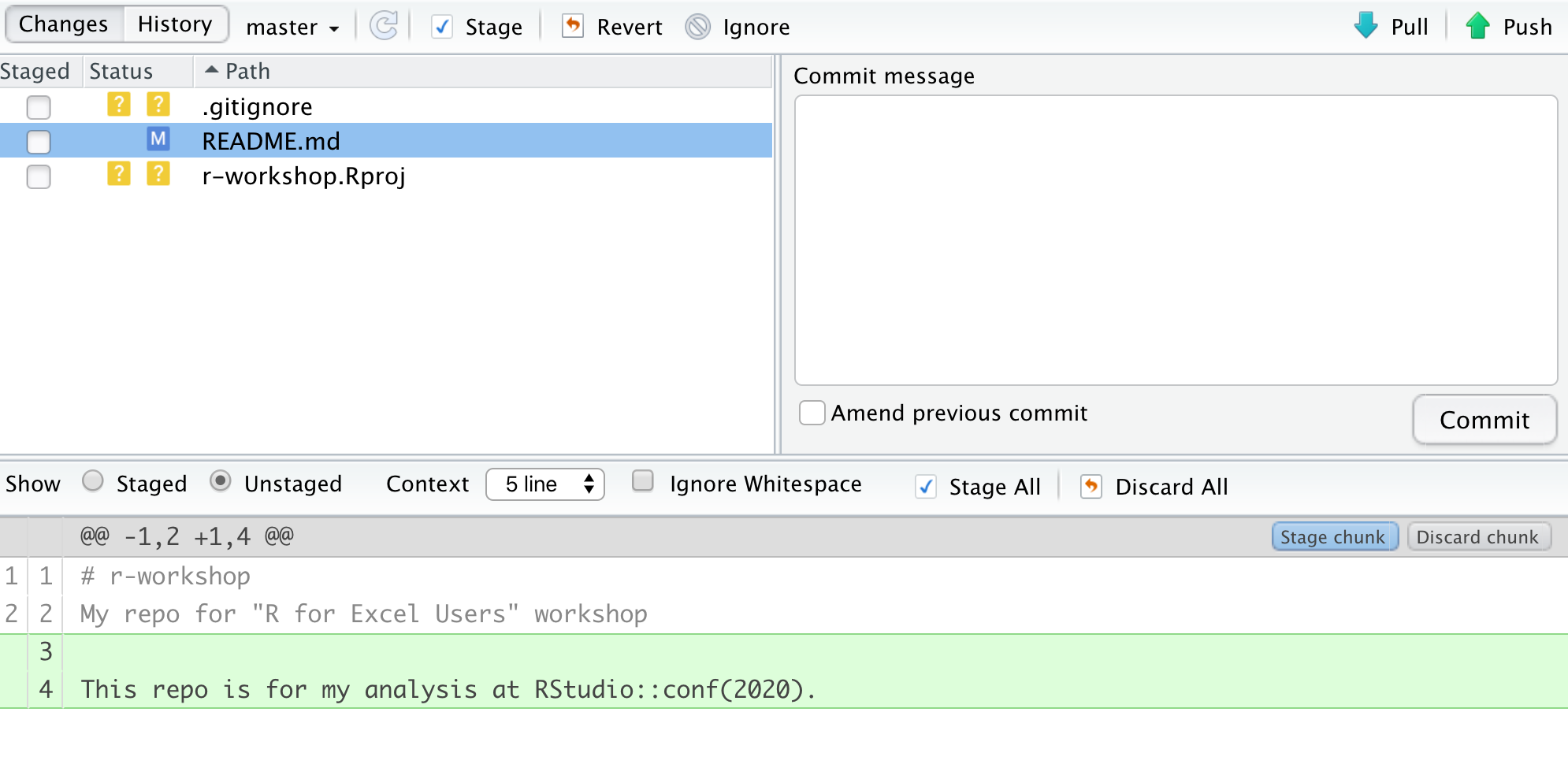
Stage
Let’s click the boxes next to each file. This is called “staging a file”: you are indicating that you want GitHub to track this file, and that you will be syncing it shortly. Notice:
- .Rproj and .gitignore files: the question marks turn into an A because these are new files that have been added to your repo (automatically by RStudio, not by you).
- README.md file: the M indicates that this was modified (by you)
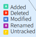
These are the codes used to describe how the files are changed, (from the RStudio cheatsheet):
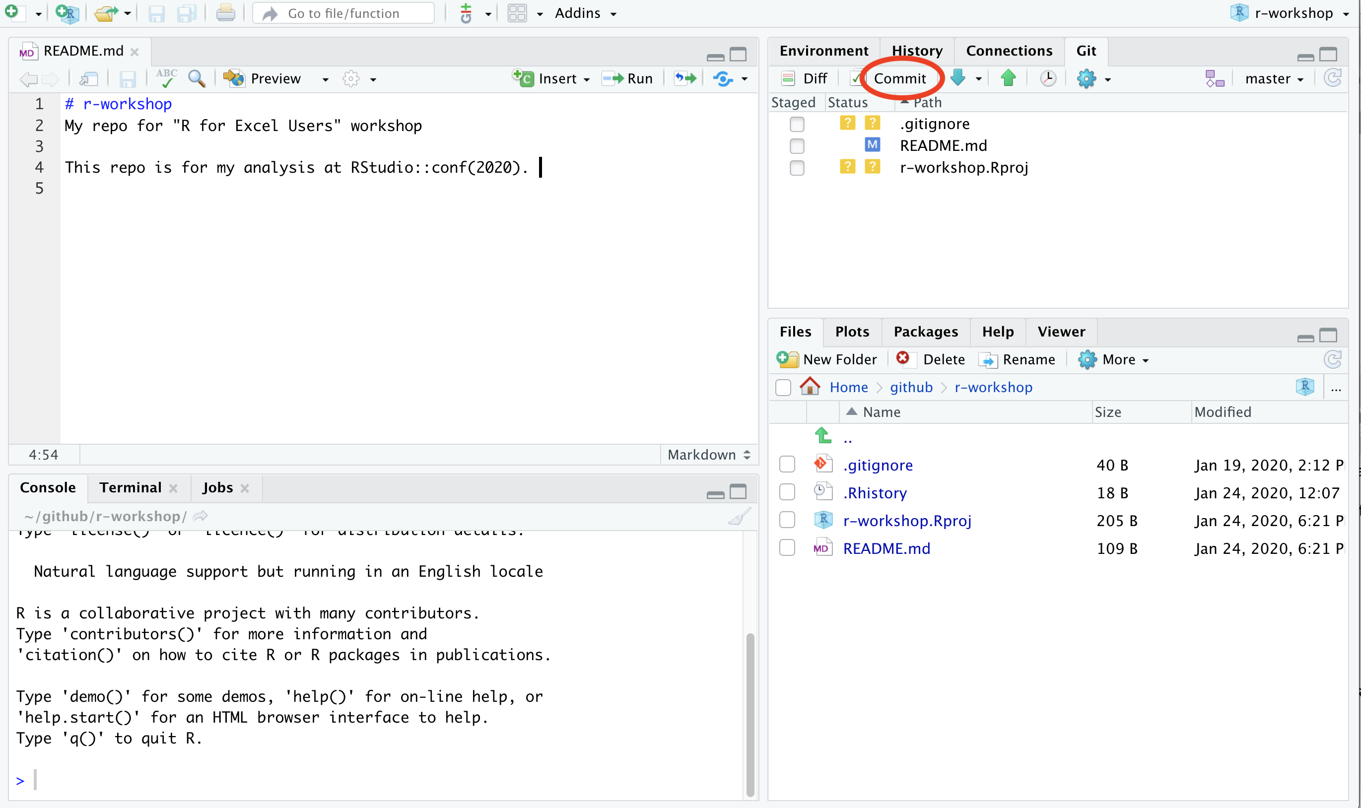
Commit
Next, we click on the Commit section.
Committing is different from saving our files (which we still have to do! RStudio will indicate a file is unsaved with red text and an asterix). We commit a single file or a group of files when we are ready to save a snapshot in time of the progress we’ve made. Maybe this is after a big part of the analysis was done, or when you’re done working for the day.
Committing our files is a 2-step process.
First, you write a “commit message”, which is a human-readable note about what has changed that will accompany GitHub’s non-human-readable alphanumeric code to track our files. I think of commit messages like breadcrumbs to my Future Self: how can I use this space to be useful for me if I’m trying to retrace my steps (and perhaps in a panic?).
Second, you press Commit.
![]()
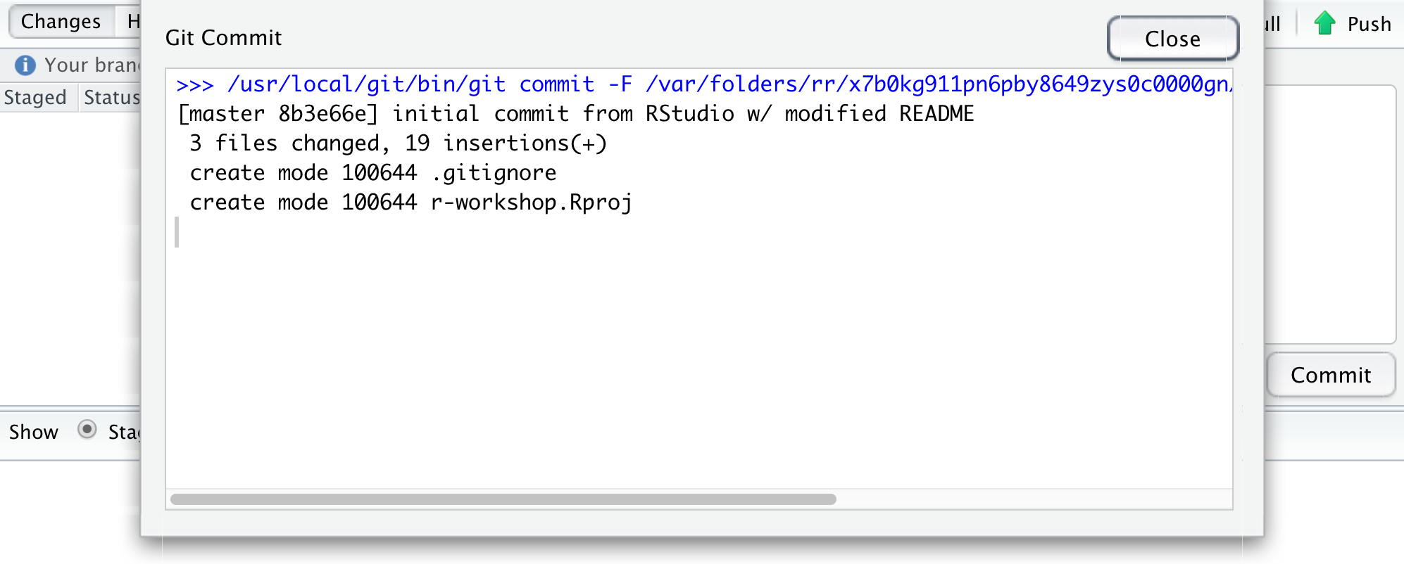
When we have committed successfully, we get a rather unsuccessful-looking pop-up message. You can read this message as “Congratulations! You’ve successfully committed 3 files, 2 of which are new!” It is also providing you with that alphanumeric SHA code that GitHub is using to track these files.
If our attempt was not successful, we will see an Error. Otherwise, interpret this message as a joyous one.
Does your pop-up message say “Aborting commit due to empty commit message.”? GitHub is really serious about writing human-readable commit messages.
When we close this window there is going to be (in my opinion) a very subtle indication that we are not done with the syncing process.
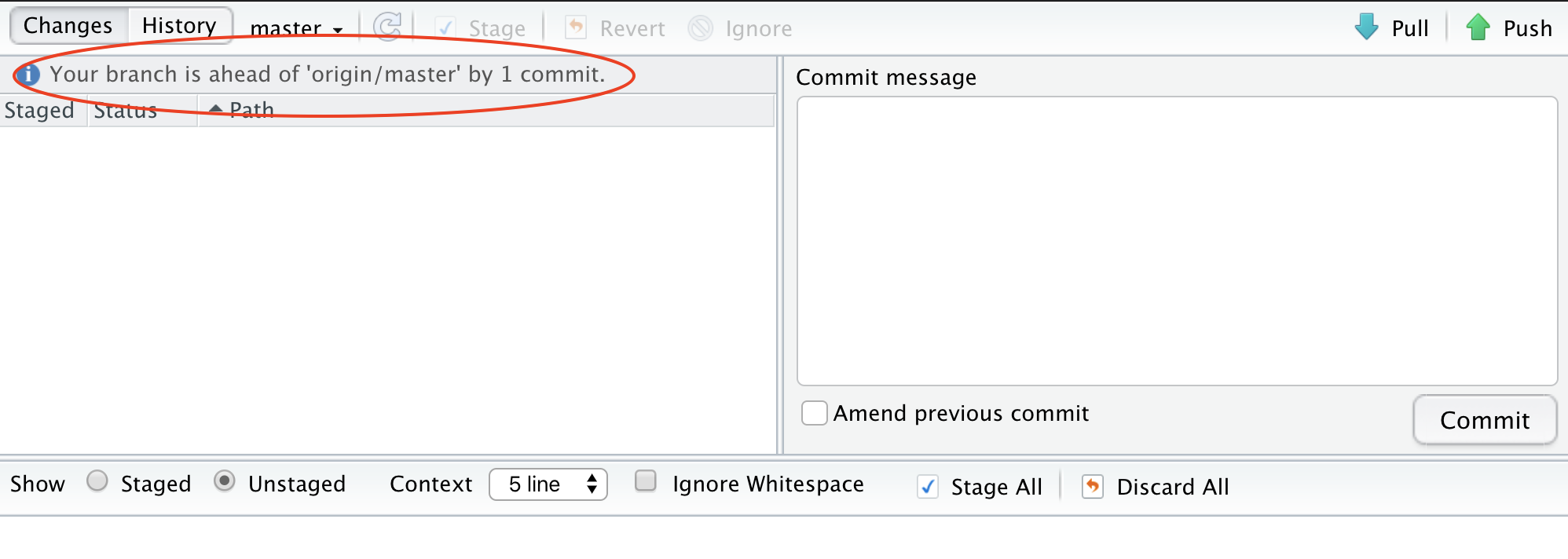
We have successfully committed our work as a breadcrumb-message-approved snapshot in time, but it still only exists locally on our computer. We can commit without an internet connection; we have not done anything yet to tell GitHub that we want this pushed to the remote repo at GitHub.com. So as the last step, we push.
Push
The last step in the syncing process is to Push!
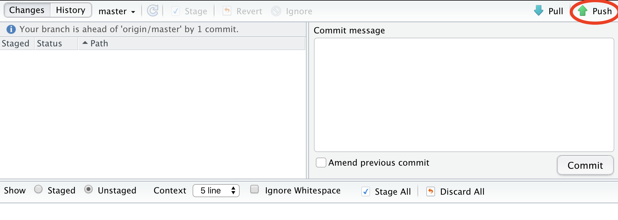
Awesome! We’re done here in RStudio for the moment, let’s check out the remote on github.com.
Commit history
The files you added should now be on github.com.
Notice how the README.md file we created is automatically displayed at the bottom. Since it is good practice to have a README file that identifies what code does (i.e. why it exists), GitHub will display a Markdown file called README nicely formatted.
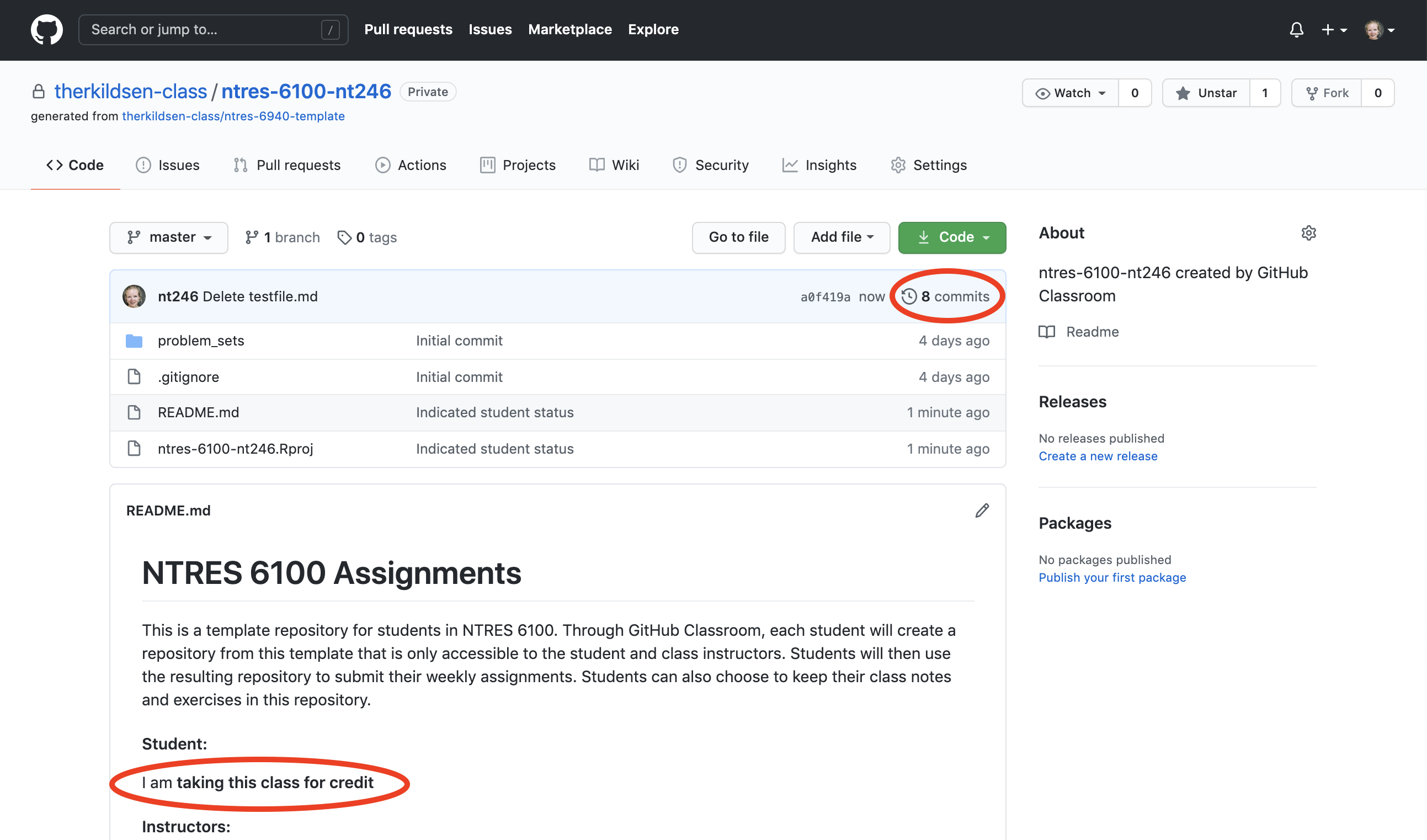
Let’s also explore the commit history. The 2 commits we’ve made (the first was when we originally initiated the repo from github.com) are there!
Project-oriented workflows
Let’s go back to RStudio and see how we set up well-organized projects and workflows for our data analyses.
This GitHub repository is now also an RStudio Project (capital P
Project). This just means that RStudio has saved this additional file
with extension .Rproj (ours is
ntres-6100-assignments-USERNAME.Rproj) to store specific
settings for this project. It’s a bit of technology to help us get into
the good habit of having a project-oriented workflow.
A project-oriented workflow means that we are going to organize all of the relevant things we need for our analyses in the same place. That means that this is the place where we keep all of our data, code, figures, notes, etc.
R Projects are great for reproducibility, because our self-contained working directory will be the first place R looks for files.
Why does this matter? It’s convenient for us to have everything associated with our analyses close at-hand. When we work with different files in R (like data or saved graphs) we always need to tell R where things “live” by identifying its file path. If files are scattered across your computer, we would have to keep track of many different filepaths. So using RStudio Projects and having a project-oriented workflow and mindset makes our analysis less brittle and more portable — across people, time, and computers. If you’re not convinced, please check Jenny Bryan’s arguments here or here and Chapter 6 in R4DS(2e).
Working directory
Now that we have our Project, let’s revisit this important question: where are we? Now we are in our Project. Everything we do will by default be saved here so all our files can be nicely organized.
And this is important because if our friend Maria clones this
repository that you just made and saves it in
Maria/my/projects/way/over/here, she will still be able to
interact with your files as you are here.
Project-oriented workflows in action (aka our analytical setup)
Let’s get a bit organized. First, let’s create a new Quarto file for notes that you want to take as we work through the different modules of this course.
Create a new Rmd file
So let’s do this (again):
File > New File > Quarto Document … (or click the green plus in the top left corner).
Let’s set up this file so it’s ready for us to enter notes into. I’m going to update the header with a new title and add my name, for now leave the output as html, and then I’m going to delete the rest of the document so that we have a clean start.
Efficiency Tip: I use Shift - Command - Down Arrow to highlight text from my cursor to the end of the document
---
title: "Notes for NTRES 6100 lectures"
author: "Nina Overgaard Therkildsen"
format: html
editor: visual
---

# Course notes
We're going to learn a lot about GitHub and the tidyverse and it's going to be fun.
Now, let’s save it. I’m going to call my file
course-notes.qmd.
Notice that when we save this file, it pops up in our Git tab. Git knows that there is something new in our repo.
Let’s also render this file. And look: Git also sees the rendered .html file.
And let’s practice syncing our file to to GitHub: pull, stage, commit, push
Troubleshooting: What if a file doesn’t show up in the Git tab and you expect that it should? Check to make sure you’ve saved the file. If the filename is red with an asterix, there have been changes since it was saved. Remember to save before syncing to GitHub!
Create data and figures folders
Let’s create a few folders to be organized. Let’s have one for our the raw data, and one for the figures we will output. We can do this in RStudio, in the bottom right pane Files pane by clicking the New Folder button:
- folder called “data”
- folder called “figures”
We can press the refresh button in the top-right of this pane (next to the “More” button) to have these show up in alphabetical order.
Now let’s go to our Finder or Windows Explorer: our new folders are there as well!
Output formats for RMarkdown
After pushing, the rendered html of course-notes.Rmd
file should show up in our GitHub repo after we push it. But how does it
look? GitHub just displays the raw html text file, not the nice-looking
rendered version we’ll see in a browser.
The nicely formatted files you see on GitHub (e.g. typical README
pages) are markdown files (.md in contrast to .Rmd). Fortunately, Quarto
can output to this format, along with several others including pdf and
word documents. We can change the output format in the YAML header at
the top of our Quarto document. For the rendered output to display
nicely on GitHub, we want to select output: gfm (GitHub
Flavored Markdown).
---
title: "Notes for NTRES 6100 lectures"
author: "Nina Overgaard Therkildsen"
format: gfm
editor: visual
---
You can find much more information about Quarto output formats here. For most of
our work in this course, we will want to use the gfm output
type because this displays nicely on the GitHub website.
Move files to data folder
Now let’s try adding a file to our local RStudio project folder so we can push it to GitHub. One of the data files you will need for your next problem set is located here. Save this file (using the “Download raw file” icon in the top right of the file display area) into the ‘data’ subfolder of your R project (the folder you have created for the project (in the cloning process) on your local computer).
Now let’s go back to RStudio. We can click on the data folder in the Files tab and now see this new file.
The data folder also shows up in your Git tab. But the figures folder does not. That is because GitHub cannot track an empty folder, it can only track files within a folder.
Let’s sync the data file (we will be able to sync the figures folder after we’ve generated some plots later in the course). We can stage multiple files at once by typing Command - A and clicking “Stage” (or using the space bar). To Sync: pull - stage - commit - push!
Activity
Edit your README either directly on GitHub or in RStudio and practice syncing (pull, stage, commit, push). For example,
- Indicate whether you’re taking the course for credit
- Add a fun fact about yourself
- Add another line of text
- Add a picture of yourself (see instructions from last class here)
Explore your Commit History
Committing - how often? Tracking changes in your files
Whenever you make changes to the files in GitHub, you will walk through the Pull -> Stage -> Commit -> Push steps.
I tend to do this every time I finish a task (basically when I start getting nervous that I will lose my work). Once something is committed, it is very difficult to lose it.
Adding version control to a pre-existing R-project
You may have been working on an RStudio project earlier and now you want to add version control through GitHub. You can easily set that up with these instructions by from Happy Git with R by Jenny Bryan. In fact, we will do this for our Assignment 2!