Lesson 10: Tidy Data
Readings
Required:
Chapter 5 in in R for Data Science (2e) by Hadley Wickham, Mine Çetinkaya-Rundel & Garrett Grolemund
This cool Twitter thread by Julia Lowndes and Allison Horst. If you can’t access the thread or want more detail, the same material is expanded upon on Julie’s Openscapes website. Openscapes is an awesome organization that champions open practices in environmental science - check it out!
Additional resources:
- Jenny
Bryan’s Intro to Tidy Data
- the repo this links to has some useful exercises too, but uses the
outdated
spread()andgather()functions so don’t get confused by the code.
- the repo this links to has some useful exercises too, but uses the
outdated
tidyrvignette on tidy data
- Hadley’s paper on tidy data provides a thorough investigation
Announcements
Assignment 4 due tonight - submit by pushing to your class GitHub repo
We’re half way through the course! We will send out a link to a mid-term evaluation form (we’ll use our own form because the official CALS version won’t be ready in time to work with our schedule). We would appreciate your candid feedback so we can make the most of our remaining time together. All responses are completely anonymous.
Your GitHub PAT (personal access token) may expire soon (if you had set it to 30 days). We’ll review how to renew it at the end of class
Learning objectives
So far, we’ve only worked with data that were already formatted for efficient processing with tidyverse functions. In this session we’ll learn some tools to help get data into that format - make it tidy and more coder-friendly.
By the end of today’s class, you should be able to:
- Describe the concept of tidy data
- Determine whether a dataset is in tidy format
- Use
tidyr::pivot_wider()andtidyr::pivot_longer()to reshape data frames - Use
tidyr::unite()andtidyr::separate()to merge or separate information from different columns
Acknowledgements
Todays lesson integrates material from multiple sources, including the excellent R for Excel users course by Julia Stewart Lowndes and Allison Horst and several other sources specified below.
Set-up for today’s exercises
Create a new R script and load packages
Open the R Project associated with your personal class GitHub repository.
PULL to make sure your project is up to date
Create a new R script file and save it as
my_tidying.RmdLoad the
tidyversepackage
# Load packages
library(tidyverse)
What is tidy data?
“Tidy” might sound like a generic way to describe non-messy looking data, but it actually refers to a specific data structure.
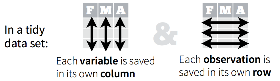
A data set is tidy if:
- Each column is a variable;
- Each row is an observation;
- Each cell is a value.
See: Ch. 12 in R for Data Science by Grolemund & Wickham.
An implication of this definition is that each value belongs to exactly one variable and one observation. This also means that tidy data is relative, as it depends on how you define your observational unit and variables.
A key idea here is that instead of building your analyses around whatever (likely weird) format your data are in, take deliberate steps to make your data tidy. When your data are tidy, you can use a growing assortment of powerful analytical and visualization tools instead of inventing home-grown ways to accommodate your data. This will save you time since you aren’t reinventing the wheel, and will make your work more clear and understandable to your collaborators (most importantly, Future You).
Note that to effectively use ggplot() your data must be
in tidy format. It also makes it easier to take advantage of R’s
vectorized nature (most built-in R functions work with vectors of
values)
Review of the beautiful slides by Julia Lowndes and Allison Horst for a clear overview of the motivation for working with tidy data.
Let’s go through some examples to get a better understanding of what tidy data look like.
Let’s first compare the four different representations of the same dataset shown in Chapter 12.2 in Grolemund and Wickham’s “R for Data Science” including the same values of four variables country, year, population, and cases.
Which of these representations are in tidy format?
Exercise
The datasets discussed in Chapter 12 of for Data Science come with
the tidyverse package, so you can access them by just
typing their names, e.g. table1, table2 etc.
We computed the infection rate per year 10,000 people for each
year and each country from table1 together using
our now familiar dplyr wrangling tools.
Your task: Now calculate this same statistic from
table2 and table4a + table4b. You
will need to perform four operations:
- Extract the number of TB cases per country per year.
- Extract the matching population per country per year.
- Divide cases by population, and multiply by 10000.
- Store back in the appropriate place.
Which representation is easiest to work with? Which is hardest? Why?
If I had one thing to tell biologists learning bioinformatics, it would be “write code for humans, write data for computers”. — Vince Buffalo (@vsbuffalo)
Pivoting between long and wide data formats
Now that the motivation for wanting to work with data in tidy format
hopefully is clear, let’s explore some powerful functions from the
package tidyr for reshaping data. (tidyr comes
bundled with the tidyverse, so we don’t have to install it
separately).
Often, datasets will not be in tidy format because they are organized to facilitate some use other than analysis. For example, data is often organized to make entry or reading by humans as easy as possible.
This means for most real analyses, you’ll need to do some tidying. The first step is always to figure out what the variables and observations are. Sometimes this is easy; other times you’ll need to consult with the people who originally generated the data. The second step is to resolve one of two common problems:
One variable might be spread across multiple columns.
One observation might be scattered across multiple rows.
Typically a dataset will only suffer from one of these problems;
it’ll only suffer from both if you’re really unlucky! To fix these
problems, you’ll need the two most important functions in tidyr:
pivot_longer() and pivot_wider().
We’ll walk through an illustration of how to use these by following Chapter 12.3 Pivoting in Grolemund and Wickham’s “R for Data Science”.
That overview uses a simple example with a small number of variables,
so we can easily list them individually when we use
pivot_longer(). For datasets with more variables, we can
use more automated ways to index columns, the same helper functions we
used for the select() function (you can refresh your memory
here). See
examples of this in the useful tidyr
vignette on pivoting.
After reviewing the pivot functions, let’s continue on
to also take a look at Chapter
12.4 in R for Data Science on separate() and
unite() - two simple functions for splitting and combining
information from different columns.
Application to a different dataset: LOTR
To explore tidy data in a different context, let’s work through a
tutorial developed by Jenny Bryan using data on the Lord of the Rings
movies. This nicely illustrates the concepts of lengtening and widening
datasets. It uses outdated functions for pivoting the dataframes,
however, so we’ll work through updated code here (i.e. only look at the
01-intro.md file, not the 02-gather.md and
03-spread.md - we’ll work through those steps here).
First let’s read the intro (01-intro.md) here
Then let’s work through reshaping the data.
1. Import untidy Lord of the Rings data
First, we bring the data into data frames or tibbles, one per film, and do some inspection.
fship <- read_csv("https://raw.githubusercontent.com/jennybc/lotr-tidy/master/data/The_Fellowship_Of_The_Ring.csv")

ttow <- read_csv("https://raw.githubusercontent.com/jennybc/lotr-tidy/master/data/The_Two_Towers.csv")

rking <- read_csv("https://raw.githubusercontent.com/jennybc/lotr-tidy/master/data/The_Return_Of_The_King.csv")
2. Collect untidy Lord of the Rings data into a single data frame
We now have one data frame per film, each with a common set of 4
variables. Step one in tidying this data is to glue them together into
one data frame, stacking them up row wise. This is called row binding
and we use dplyr::bind_rows().
lotr_untidy <- bind_rows(fship, ttow, rking)

lotr_untidy
## # A tibble: 9 × 4
## Film Race Female Male
## <chr> <chr> <dbl> <dbl>
## 1 The Fellowship Of The Ring Elf 1229 971
## 2 The Fellowship Of The Ring Hobbit 14 3644
## 3 The Fellowship Of The Ring Man 0 1995
## 4 The Two Towers Elf 331 513
## 5 The Two Towers Hobbit 0 2463
## 6 The Two Towers Man 401 3589
## 7 The Return Of The King Elf 183 510
## 8 The Return Of The King Hobbit 2 2673
## 9 The Return Of The King Man 268 24593. Tidy the untidy Lord of the Rings data
We are still violating one of the fundamental principles of
tidy data. “Word count” is a fundamental variable in
our dataset and it’s currently spread out over two variables,
Female and Male. Conceptually, we need to
gather up the word counts into a single variable and create a new
variable, Gender, to track whether each count refers to
females or males. We use the pivot_longer() function from
the tidyr package to do this.
lotr_tidy <-
  pivot_longer(lotr_untidy, c(Male, Female), names_to = 'Gender', values_to = 'Words')

lotr_tidy
## # A tibble: 18 × 4
## Film Race Gender Words
## <chr> <chr> <chr> <dbl>
## 1 The Fellowship Of The Ring Elf Male 971
## 2 The Fellowship Of The Ring Elf Female 1229
## 3 The Fellowship Of The Ring Hobbit Male 3644
## 4 The Fellowship Of The Ring Hobbit Female 14
## 5 The Fellowship Of The Ring Man Male 1995
## 6 The Fellowship Of The Ring Man Female 0
## 7 The Two Towers Elf Male 513
## 8 The Two Towers Elf Female 331
## 9 The Two Towers Hobbit Male 2463
## 10 The Two Towers Hobbit Female 0
## 11 The Two Towers Man Male 3589
## 12 The Two Towers Man Female 401
## 13 The Return Of The King Elf Male 510
## 14 The Return Of The King Elf Female 183
## 15 The Return Of The King Hobbit Male 2673
## 16 The Return Of The King Hobbit Female 2
## 17 The Return Of The King Man Male 2459
## 18 The Return Of The King Man Female 268Tidy data… mission accomplished!
To explain our call to pivot_longer() above, let’s read
it from right to left: we took the variables Female and
Male and gathered their values into a single new variable
Words. This forced the creation of a companion variable
Gender, which tells whether a specific value of
Words came from Female or Male. All other variables, such
as Film, remain unchanged and are simply replicated as
needed.
4. OPTIONAL: Write the tidy data to a delimited file
Now we write this multi-film, tidy dataset to file for use in various downstream scripts for further analysis and visualization.
write_csv(lotr_tidy, file = "datasets/lotr_tidy.csv")Your turn
After tidying the data and completing your analysis, you may want to output a table that has each race in its own column. Let’s use the
pivot_wider()function to make such a table and save it as “lotr_wide”OPTIONAL: Use the
pivot_longer()function to transform you lotr_wide back to tidy format.
click to see our approach
# let's get one variable per Race
lotr_tidy |>
  pivot_wider(names_from = Race, values_from = Words)
## # A tibble: 6 × 5
## Film Gender Elf Hobbit Man
## <chr> <chr> <dbl> <dbl> <dbl>
## 1 The Fellowship Of The Ring Male 971 3644 1995
## 2 The Fellowship Of The Ring Female 1229 14 0
## 3 The Two Towers Male 513 2463 3589
## 4 The Two Towers Female 331 0 401
## 5 The Return Of The King Male 510 2673 2459
## 6 The Return Of The King Female 183 2 268# let's get one variable per Gender
lotr_tidy |>
pivot_wider(names_from = Gender, values_from = Words)## # A tibble: 9 × 4
## Film Race Male Female
## <chr> <chr> <dbl> <dbl>
## 1 The Fellowship Of The Ring Elf 971 1229
## 2 The Fellowship Of The Ring Hobbit 3644 14
## 3 The Fellowship Of The Ring Man 1995 0
## 4 The Two Towers Elf 513 331
## 5 The Two Towers Hobbit 2463 0
## 6 The Two Towers Man 3589 401
## 7 The Return Of The King Elf 510 183
## 8 The Return Of The King Hobbit 2673 2
## 9 The Return Of The King Man 2459 268# let's get one variable per combo of Race and Gender
lotr_tidy |>
unite(Race_Gender, Race, Gender) |>
pivot_wider(names_from = Race_Gender, values_from = Words)## # A tibble: 3 × 7
## Film Elf_Male Elf_Female Hobbit_Male Hobbit_Female Man_Male Man_Female
## <chr> <dbl> <dbl> <dbl> <dbl> <dbl> <dbl>
## 1 The Fellows… 971 1229 3644 14 1995 0
## 2 The Two Tow… 513 331 2463 0 3589 401
## 3 The Return … 510 183 2673 2 2459 268More exercises on the LOTR data (you can do these on your own later)
The word count data is given in two untidy and gender-specific files available at these URLs:
https://raw.githubusercontent.com/jennybc/lotr-tidy/master/data/Female.csv
https://raw.githubusercontent.com/jennybc/lotr-tidy/master/data/Male.csv
Write an R script that reads them in and writes a single tidy data frame to file. Literally, reproduce the lotr_tidy data frame and the lotr_tidy.csv data file from above.
Write R code to compute the total number of words spoken by each race across the entire trilogy. Do it two ways:
- Using film-specific or gender-specific, untidy data frames as the input data.
- Using the lotr_tidy data frame (that we generated above) as input.
Reflect on the process of writing this code and on the code itself. Which is easier to write? Easier to read?
Write R code to compute the total number of words spoken in each film. Do this by copying and modifying your own code for totalling words by race. Which approach is easier to modify and repurpose – the one based on multiple, untidy data frames or the tidy data?
Application to our coronavirus dataset
Let’s now return to our Coronavirus dataset. Let’s remind ourselves of it’s structure
coronavirus <- read_csv('https://raw.githubusercontent.com/RamiKrispin/coronavirus/master/csv/coronavirus.csv')

coronavirus
## # A tibble: 919,308 × 15
## date province country lat long type cases uid iso2 iso3 code3
## <date> <chr> <chr> <dbl> <dbl> <chr> <dbl> <dbl> <chr> <chr> <dbl>
## 1 2020-01-22 Alberta Canada 53.9 -117. confir… 0 12401 CA CAN 124
## 2 2020-01-23 Alberta Canada 53.9 -117. confir… 0 12401 CA CAN 124
## 3 2020-01-24 Alberta Canada 53.9 -117. confir… 0 12401 CA CAN 124
## 4 2020-01-25 Alberta Canada 53.9 -117. confir… 0 12401 CA CAN 124
## 5 2020-01-26 Alberta Canada 53.9 -117. confir… 0 12401 CA CAN 124
## 6 2020-01-27 Alberta Canada 53.9 -117. confir… 0 12401 CA CAN 124
## 7 2020-01-28 Alberta Canada 53.9 -117. confir… 0 12401 CA CAN 124
## 8 2020-01-29 Alberta Canada 53.9 -117. confir… 0 12401 CA CAN 124
## 9 2020-01-30 Alberta Canada 53.9 -117. confir… 0 12401 CA CAN 124
## 10 2020-01-31 Alberta Canada 53.9 -117. confir… 0 12401 CA CAN 124
## # ℹ 919,298 more rows
## # ℹ 4 more variables: combined_key <chr>, population <dbl>,
## # continent_name <chr>, continent_code <chr>QUESTION: Is this in tidy format?
Similar to what we did in the last class, we could visualize the global sums for the different types of case counts by date (note that in August 2021, the dataset stopped tracking recoveries)
coronavirus |>
  filter(cases > 0) |>
  group_by(date, type) |>
  summarize(cases = sum(cases)) |>
  ggplot() +
  geom_col(aes(x = date, y = cases, fill = type))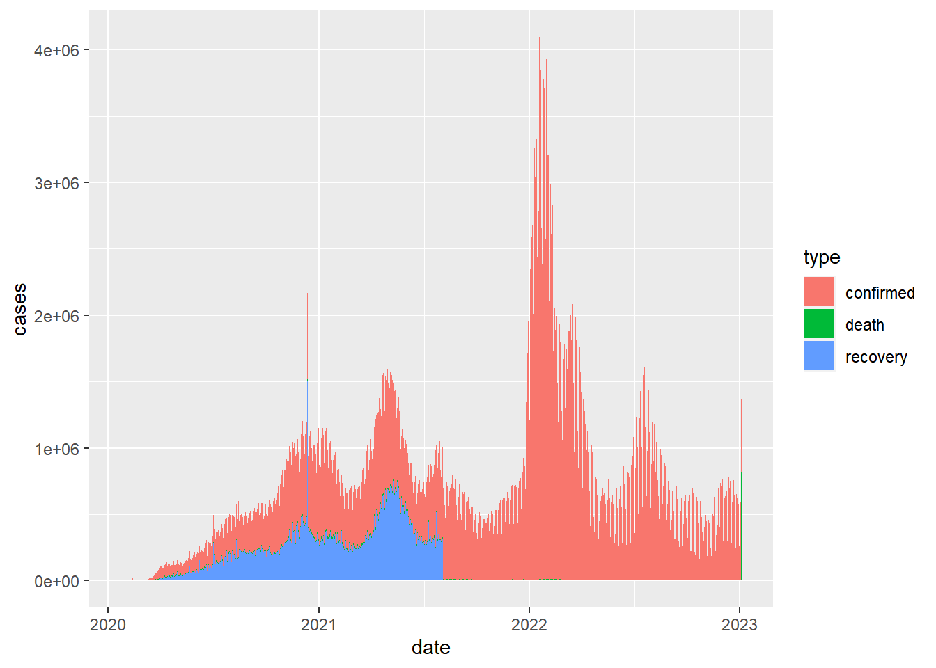
Let’s see how we would do that if the data had been in a wider format.
Your turn
Convert the coronavirus dataset to a wider format where the confirmed cases, deaths and recovered cases are shown in separate columns.
click to see our approach
# Let's just select a few key columns so we better can follow what happens to the data structure
corona_wide <- coronavirus |>
  select(date, country, province, type, cases) |>
  pivot_wider(names_from = type, values_from = cases)
Now how do we reproduce the barchart of total cases per day broken down by type?
And how would we plot the daily counts of different case types within a country?
With the long format this is easy:
coronavirus |>
  filter(cases > 0, country == "US") |>
  ggplot() +
  geom_line(aes(x = date, y = cases, color = type))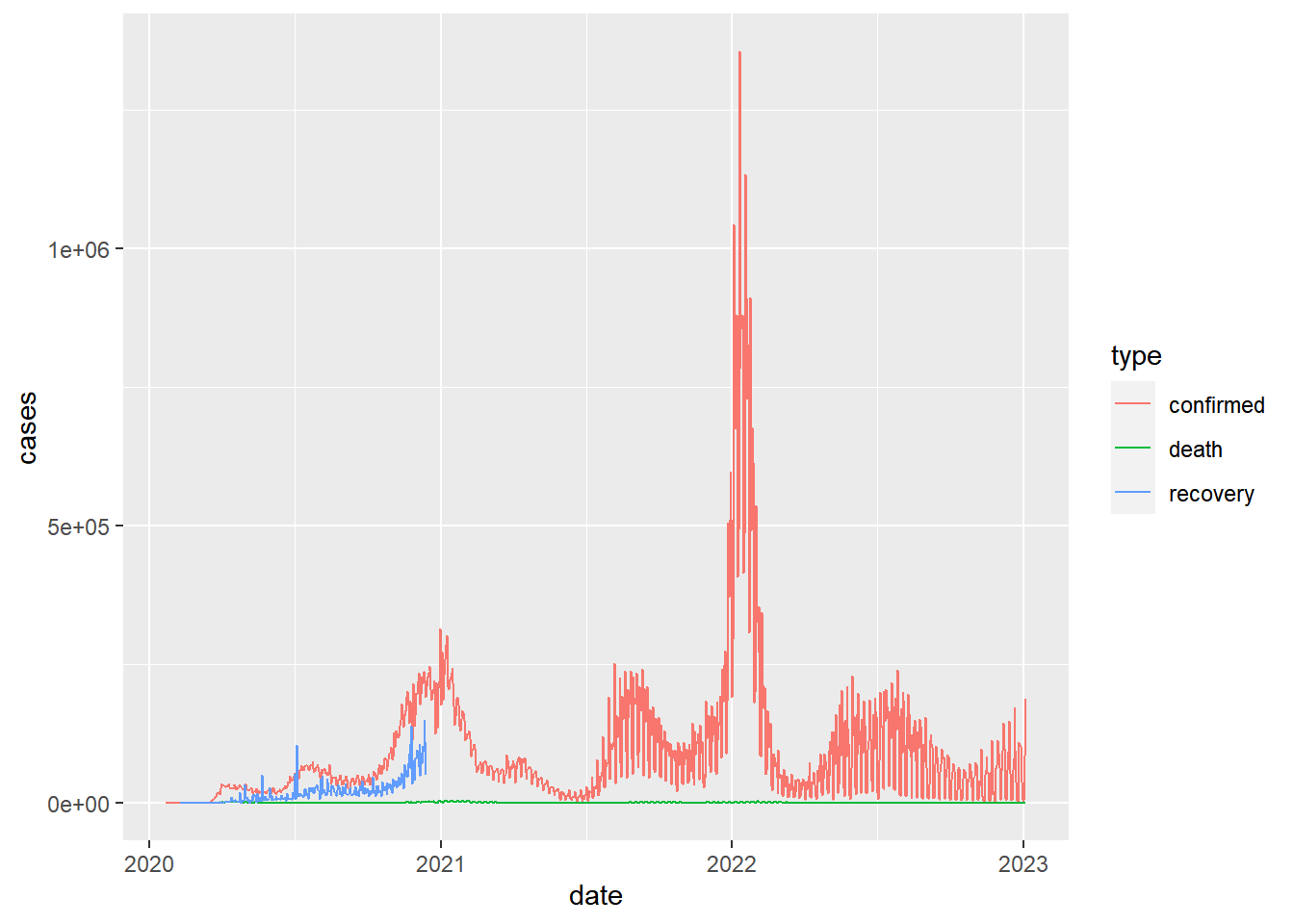
How would we do this with the coronavirus_wide format?
That would be much more difficult.
As mentioned above, however, there are plot types where the wide
format provides the best input. In an earlier class, for example, I
showed the example of plotting the total death count per country against
the total count of confirmed cases. It would be cumbersome to pull these
out of the long format because in ggplot we are mapping
variables to aesthetics and now we want to map
different levels of a variable to different aesthetics. So let’s make
those different levels separate variables by widening the data.
coronavirus_ttd <- coronavirus |>
  group_by(country, type) |>
  summarize(total_cases = sum(cases)) |>
  pivot_wider(names_from = type, values_from = total_cases)

# Now we can plot this easily
ggplot(coronavirus_ttd) +
  geom_label(mapping = aes(x = confirmed, y = death, label = country))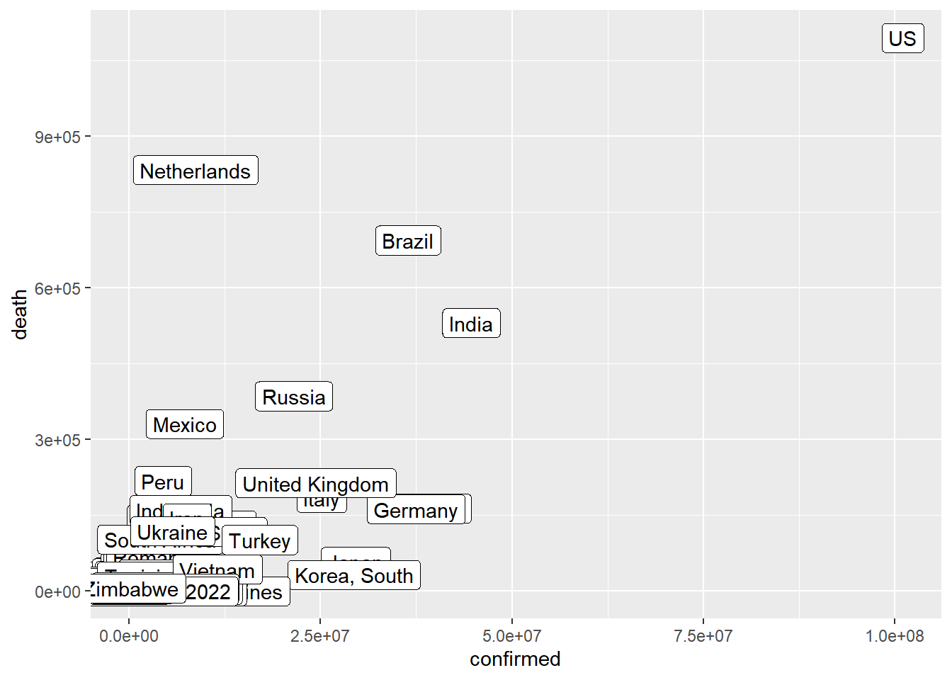
This case highlights how the definition of what a variable and an observation is context-dependent so different formats of the same data can be considered tidy based on how we are thinking about the data and we may need to switch back and forth between long and wide formats to explore different levels of a dataset.
Before we wrap up - Renew our GitHub access token
When we configured git to connect with our GitHub account through RStudio, many of you may have used a PAT (personal access token) that was only valid for 30 days. Let’s revisit how we can set up with a new token by working through the procedures described in Lesson 2.