Lesson 16: Functions

Readings

Required:

• Chapter 19 in R for Data Science by Hadley Wickham & Garrett Grolemund

Other resources:

• Chapters 18-21 in Jenny Bryan’s STAT545 notes

Announcements

• We’re getting towards the end of the course - only three more classes left
• You will be giving your 1.5 minute end-of-class student presentations next Thursday (March 30). The presentations are part of the requirements to pass the course. Auditors are encouraged, but not required, to present.

Today’s learning objectives

Today, we will cover a brief introduction to how to write your own functions in R.

By the end of today’s class, you should be able to:

• Write a simple function to automate a task
• Set default values for function arguments
• Explain why we should divide code into small, single-purpose functions

Getting started with functions

As always, we’ll need the tidyverse, so let’s start by loading that in

library(tidyverse)

We will first introduce functions with these slides

Then we’ll illustrate how to write a basic function with an example slightly modified from the Data Carpentry’s semester program lecture notes.

The basic syntax

function_name <- function(inputs) {
  output_value <- do_something(inputs)
  return(output_value)
}

Here is an example of a function that will calculate the volume of a shrub.

calc_shrub_vol <- function(length, width, height) {
  area <- length * width
  volume <- area * height
  return(volume)
}

When we run this code, nothing seems to happen (we don’t get any output). Creating a function doesn’t run it. But it stores it, so that we can run it later with some arguments (or without arguments if the function has specified defaults - more about this later). Let’s assume that we’ve measured a shrub. Its length is 0.8, its width is 1.6, and its height is 2.0. We can now call our function with these numbers (entering each number at the relevant position, according to how arguments were listed when we defined the function (in this case length, width, height)).

calc_shrub_vol(0.8, 1.6, 2.0)

## [1] 2.56

This code will just print the results to our console. We can also store the output for later use.

shrub_vol <- calc_shrub_vol(0.8, 1.6, 2.0)

Your turn: Exercise

Copy the following function into your R script and replace the ________ with variables names for the input and output.

convert_pounds_to_grams <- function(________) {
    grams <- 453.6 * pounds
    return(________)
}

Use the function to calculate how many grams there are in 3.75 pounds.

Objects defined within functions

It is important to note that even after we’ve defined and run a function, we can’t access variables created inside the function. For example

volume
> object 'volume' not found

width
> object 'width' not found

Default arguments

Defaults can be set for common inputs. For example, many of our shrubs are the same height so for those shrubs we only measure the length and width. So we want a default value for the height for cases where we don’t measure it. We can over-write the default if we specify something different for height, but if we don’t specify a value for this argument, the default will be used.

calc_shrub_vol <- function(length, width, height = 1) {
  area <- length * width
  volume <- area * height
  return(volume)
}

calc_shrub_vol(0.8, 1.6)

## [1] 1.28

calc_shrub_vol(0.8, 1.6, 2.0)

## [1] 2.56

calc_shrub_vol(length = 0.8, width = 1.6, height = 2.0)

## [1] 2.56

Named vs unnamed arguments

When to use or not use argument names. For example, we can call our function either by explicitly naming each of our arguments or just list them by position

calc_shrub_vol(length = 0.8, width = 1.6, height = 2.0)

OR

calc_shrub_vol(0.8, 1.6, 2.0)

You can always name your arguments (i.e. length = 0.8 instead of just 0.8). The value will get assigned to the argument of that name. When you’re naming each argument, the order in which you list them does not matter.

If you’re not naming your arguments (i.e. just 0.8 instead of length = 0.8), then order determines what argument each value gets assigned to. Here, the first listed value will be assigned to length, the second to width, and the third to height. If the order is hard to remember, name your arguments.

In many cases there are a lot of optional arguments (arguments that have defaults defined so that they don’t need to be specified for the function to run). Convention to always name optional arguments. So, in our case, the most common approach would be

calc_shrub_vol(0.8, 1.6, height = 2.0)

## [1] 2.56

Combining functions

Each function should be single conceptual chunk of code. Functions can be combined to do larger tasks in two ways.

The first is to call multiple functions in a row

est_shrub_mass <- function(volume){
  mass <- 2.65 * volume^0.9
  return(mass)
}

shrub_volume <- calc_shrub_vol(0.8, 1.6, 2.0)
shrub_mass <- est_shrub_mass(shrub_volume)

We can also use pipes with our own functions. The output from the first function becomes the first argument for the second function

library(dplyr)

shrub_mass <- calc_shrub_vol(0.8, 1.6, 2.0) %>%
  est_shrub_mass()

We can also nest functions, like this:

shrub_mass <- est_shrub_mass(calc_shrub_vol(0.8, 1.6, 2.0))

We can also call functions from inside other functions. This allows organizing function calls into logical groups, like this:

est_shrub_mass_from_raw <- function(length, width, height){
  volume = calc_shrub_vol(length, width, height)
  mass <- est_shrub_mass(volume)
  return(mass)
}

est_shrub_mass_from_raw(0.8, 1.6, 2.0)

An example application

Last week, we developed a for loop to create a plot for every country in a list of countries. We can re-write the plotting operation as a function that we can call for specific countries.

To try that, we’ll first need to load the gapminder dataset back in:

library(gapminder) #install.packages("gapminder")

gapminder

To simplify the code, let’s go back to what our loop looked like before we added the conditional statements:

dir.create("figures") 
dir.create("figures/Europe") 

## create a list of countries. Calculations go here, not in the for loop
gap_europe <- gapminder %>%
  filter(continent == "Europe") %>%
  mutate(gdpTot = gdpPercap * pop)

country_list <- unique(gap_europe$country) # ?unique() returns the unique values

for (cntry in country_list) { # (cntry = country_list[1])
  
  ## filter the country to plot
  gap_to_plot <- gap_europe %>%
    filter(country == cntry)
  
  ## add a print message to see what's plotting
  print(paste("Plotting", cntry))
  
  ## plot
  my_plot <- ggplot(data = gap_to_plot, aes(x = year, y = gdpTot)) + 
    geom_point() +
    ## add title and save
    labs(title = paste(cntry, "GDP per capita", sep = " "))
  
  ggsave(filename = paste("figures/Europe/", cntry, "_gdpTot.png", sep = ""), plot = my_plot)
} 

Now, we can change this into a function in the following way:

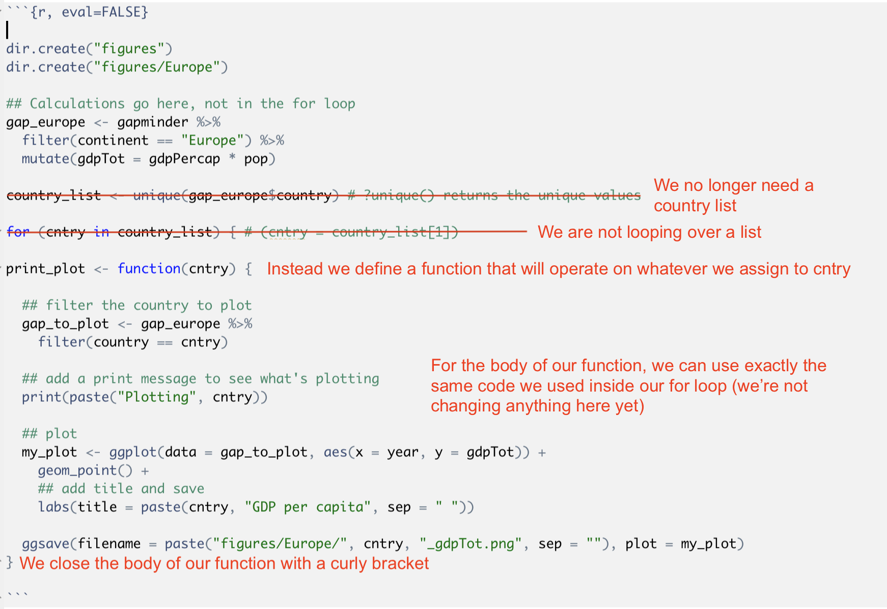
Here is our function:

dir.create("figures") 
dir.create("figures/Europe") 

## We still keep our calculation outside the function because we can do this as a single step for all countries outside the function. But we could also build this step into our function if we prefer.
gap_europe <- gapminder %>%
  filter(continent == "Europe") %>%
  mutate(gdpTot = gdpPercap * pop)

#define our function
save_plot <- function(cntry) {
  
  ## filter the country to plot
  gap_to_plot <- gap_europe %>%
    filter(country == cntry)
  
  ## add a print message to see what's plotting
  print(paste("Plotting", cntry))
  
  ## plot
  my_plot <- ggplot(data = gap_to_plot, aes(x = year, y = gdpTot)) + 
    geom_point() +
    ## add title and save
    labs(title = paste(cntry, "GDP per capita", sep = " "))
  
  ggsave(filename = paste("figures/Europe/", cntry, "_gdpTot.png", sep = ""), plot = my_plot)
} 

We can now run this function on specific countries

save_plot("Germany")
save_plot("France")

# We can even write a for loop to run the function on each country in a list of countries (doing exactly the same as our for loop did before, but now we have pulled the code specifying the operation out of the for loop itself)

country_list <- unique(gap_europe$country) # ?unique() returns the unique values

for (cntry in country_list) {
  
  save_plot(cntry)
  
}

Now we can add some more flexibility to our function. Currently, it is written to always plot the total GDP vs. year for a country. We can change the function so that it can plot other variables on the y-axis, as specified with an additional argument we provide when we call (and define) the function.

dir.create("figures") 
dir.create("figures/Europe") 

## We still keep our calculation outside the function because we can do this as a single step for all countries outside the function. But we could also build this step into our function if we prefer.
gap_europe <- gapminder %>%
  filter(continent == "Europe") %>%
  mutate(gdpTot = gdpPercap * pop)

#define our function
save_plot <- function(cntry, stat) {   # Here I'm adding an additional argument to the function, which we'll use to specify what statistic we want plotted
  
  ## filter the country to plot
  gap_to_plot <- gap_europe %>%
    filter(country == cntry)
  
  ## add a print message to see what's plotting
  print(paste("Plotting", cntry))
  
  ## plot
  my_plot <- ggplot(data = gap_to_plot, aes(x = year, y = get(stat))) +    # We need to use get() here to access the value we store as stat when we call the function
    geom_point() +
    ## add title and save
    labs(title = paste(cntry, stat, sep = " "), y = stat)
  
  ggsave(filename = paste("figures/Europe/", cntry, "_", stat, ".png", sep = ""), plot = my_plot)
} 


# Let's try calling the function with different statistics and check the outputs

save_plot("Germany", "gdpPercap")
save_plot("Germany", "pop")
save_plot("Germany", "lifeExp")

This seems to work well. But what happens if we forget to specify the statistic we want plotted?

save_plot("Germany")

We get an error message saying “argument”stat” is missing, with no default”. We can build in a default the following way:

#define our function
save_plot <- function(cntry, stat = "gdpPercap") {  

Now, if we don’t specify the statistic we want plotted, the function will execute with this specified default option. The default gets “overwritten” if we do specify a stat when we call the function.

dir.create("figures") 
dir.create("figures/Europe") 

## We still keep our calculation outside the function because we can do this as a single step for all countries outside the function. But we could also build this step into our function if we prefer.
gap_europe <- gapminder %>%
  filter(continent == "Europe") %>%
  mutate(gdpTot = gdpPercap * pop)

#define our function
save_plot <- function(cntry, stat = "gdpPercap") {   # Here I'm adding an additional argument to the function, which we'll use to specify what statistic we want plotted
  
  ## filter the country to plot
  gap_to_plot <- gap_europe %>%
    filter(country == cntry)
  
  ## add a print message to see what's plotting
  print(paste("Plotting", cntry))
  
  ## plot
  my_plot <- ggplot(data = gap_to_plot, aes(x = year, y = get(stat))) +    # We need to use get() here to access the value we store as stat when we call the function
    geom_point() +
    ## add title and save
    labs(title = paste(cntry, stat, sep = " "), y = stat)
  
  ggsave(filename = paste("figures/Europe/", cntry, "_", stat, ".png", sep = ""), plot = my_plot)
} 


# Let's try calling the function with and without specifying a statistic to plot and check the outputs

save_plot("Germany")
save_plot("Germany", "lifeExp")

Your turn

We’ve talked about how we can change the file type that ggsave() will output just by changing the extension of the specified name we want to give the file. It works like this:

# To save a .png file
ggsave(filename = "figures/Europe/Germany_gdpPercap.png", plot = my_plot)

# To save a .jpg file
ggsave(filename = "figures/Europe/Germany_gdpPercap.jpg", plot = my_plot)

# To save a .pdf file
ggsave(filename = "figures/Europe/Germany_gdpPercap.pdf", plot = my_plot)

Your task: Add an argument to our function that specifies the file type you want for the plot and edit the function so that it will output the requested file type. You can also specify a default file type that the function will use if you don’t specify a file type when you call it.

If you have more time, you can also add an additional argument that specifies the plot type (x-y scatter, line plot etc) and adjust the function to accommodate this.

Answer

click to see our approach

dir.create("figures") 
dir.create("figures/Europe") 

## We still keep our calculation outside the function because we can do this as a single step for all countries outside the function. But we could also build this step into our function if we prefer.
gap_europe <- gapminder %>%
  filter(continent == "Europe") %>%
  mutate(gdpTot = gdpPercap * pop)

#define our function
save_plot <- function(cntry, stat = "gdpPercap", filetype = "pdf") {   # Here I'm adding additional arguments to the function, which we'll use to specify what statistic we want plotted and what filetype we want
  
  ## filter the country to plot
  gap_to_plot <- gap_europe %>%
    filter(country == cntry)
  
  ## add a print message to see what's plotting
  print(paste("Plotting", cntry))
  
  ## plot
  my_plot <- ggplot(data = gap_to_plot, aes(x = year, y = get(stat))) +    # We need to use get() here to access the value we store as stat when we call the function
    geom_point() +
    ## add title and save
    labs(title = paste(cntry, stat, sep = " "), y = stat)
  
  ggsave(filename = paste("figures/Europe/", cntry, "_", stat, ".", filetype, sep = ""), plot = my_plot)
} 


# Testing our function
save_plot("Germany")
save_plot("Germany", "lifeExp", "jpg")

Testing your functions

If there is time, we’ll walk through part of the example in Chapters 18-21 in Jenny Bryan’s STAT545 notes

Example code and good advice on functions

Check out this post