Lesson 6: Plotting with ggplot, part 1
Readings
Additional resources:
The book ggplot2: Elegant Graphics for Data Analysis by Hadley Wickham, Danielle Navarro, and Thomas Lin Pedersen
Announcements
- Make sure you have a partner for Assignment 3. If you need a new
partner, just let us know in the
assignmentchannel on Slack
- As you’re working with your partner on the assignment, we encourage you to play around with avoiding and resolving merge conflicts. It’s always good to get more practice
- You’ll “submit” Assignment 3 by adding the URL to your website to the README file of your class GitHub repo
First, a quick wrap-up of our GitHub section
GitHub has powerful infrastructure for communicating with your collaborators (and yourself!) directly in your repo. It can be very helpful to have discussions about data or analysis tasks/choices right there with the rest of your project files instead of burried away in long email chains or in unrecorded verbal converasation. We’ll do a quick demo of a few of the ways you can communicate on GitHub. If you’re interested, take a look at this chapter by Julia Lowndes on using GitHub issues, or the GitHub Guide.
Now on to today’s topic…
Learning objectives for today’s class
By the end of this class you will be able to:
- Inspect your data in RStudio
- Build several common types of graphs in
ggplot2
- Customize
ggplot2aesthetics
- Combine compatible graph types
- Split up data into faceted graphs
- Change the theme of graphs
Acknowledgements: Some content from today’s lecture is adapted from the excellent R for Excel users course by Julia Stewart Lowndes and Allison Horst and the R for Data Science book by Garrett Grolemund and Hadley Wickham.
Taking notes - remember to save your work in a script or an Quarto file
Have a look at Chapter 8 in R4DS and let’s all go ahead and change our RStudio settings to never save our workspace upon exit, as shown there.
Create an R script or a Quarto file for working along with examples and doing exercises in this lecture
As we start working in RStudio, we want to continue practicing how to
sync our work to GitHub. So before we start, please open the R Project
that is associated with your class repository (the name should be
ntres-6100-assignments-YOUR_USERNAME (replace YOUR_USERNAME
with your GitHub user ID). Then create a new subdirectory names
course-notes, open an R-script or a Quarto file and save it
in this subdirectory as lecture6-ggplot1.R [or whatever you
want to call it].
Getting started with data visualization
Always plot your data!
Two main goals for statistical graphics:
- To facilitate comparisons
- To identify trends
There are several ways to make plots in R. We will exclusively use
the ggplot2 package here. If you want to know more about
why we’re using ggplot2 instead of base plot, check out the
slides 21+22 from Jenny
Bryan’s ggplot tutorial
Load packages
Now we are ready to begin. ggplot2 is a graphics package
within the tidyverse. You should already have this
installed, but we need to load the tidyverse set of
packages before you can use them.
library(tidyverse)

# If you get an error message, run `install.packages("tidyverse")`
# If you get an error message talking about the `backports` package, run this first `install.packages("backports")`
Preparing to create our first ggplot2 graph
We will visualize some fuel economy data for 38 popular models of car
using the dataset mpg which is included in the
ggplot2 package.
Inspect the data frame
Before making any kind of graph, we will always need get to know our
data first. In R, data tables are most often stored as an object of the
class data.frame. There are a few different ways to inspect
these data tables.
Directly type the name of the data frame
This method works well if you run it from a Quarto file. If run in the R Console or if rendering a Quarto, it can still do a good job with small data frames, or with data frames that are of the class
tibble(we will learn more abouttibblelater in class - for now, just think of it as an upgraded type of data frame).But, if you do it with a larger, non-
tibbledata frame, it will attempt print the entire data frame on your console or your rendered output, making the result very difficult to read.## demo (compare and contrast regular data frame and tibble) mpg## # A tibble: 234 × 11 ## manufacturer model displ year cyl trans drv cty hwy fl class ## <chr> <chr> <dbl> <int> <int> <chr> <chr> <int> <int> <chr> <chr> ## 1 audi a4 1.8 1999 4 auto… f 18 29 p comp… ## 2 audi a4 1.8 1999 4 manu… f 21 29 p comp… ## 3 audi a4 2 2008 4 manu… f 20 31 p comp… ## 4 audi a4 2 2008 4 auto… f 21 30 p comp… ## 5 audi a4 2.8 1999 6 auto… f 16 26 p comp… ## 6 audi a4 2.8 1999 6 manu… f 18 26 p comp… ## 7 audi a4 3.1 2008 6 auto… f 18 27 p comp… ## 8 audi a4 quattro 1.8 1999 4 manu… 4 18 26 p comp… ## 9 audi a4 quattro 1.8 1999 4 auto… 4 16 25 p comp… ## 10 audi a4 quattro 2 2008 4 manu… 4 20 28 p comp… ## # ℹ 224 more rowscars## speed dist ## 1 4 2 ## 2 4 10 ## 3 7 4 ## 4 7 22 ## 5 8 16 ## 6 9 10 ## 7 10 18 ## 8 10 26 ## 9 10 34 ## 10 11 17 ## 11 11 28 ## 12 12 14 ## 13 12 20 ## 14 12 24 ## 15 12 28 ## 16 13 26 ## 17 13 34 ## 18 13 34 ## 19 13 46 ## 20 14 26 ## 21 14 36 ## 22 14 60 ## 23 14 80 ## 24 15 20 ## 25 15 26 ## 26 15 54 ## 27 16 32 ## 28 16 40 ## 29 17 32 ## 30 17 40 ## 31 17 50 ## 32 18 42 ## 33 18 56 ## 34 18 76 ## 35 18 84 ## 36 19 36 ## 37 19 46 ## 38 19 68 ## 39 20 32 ## 40 20 48 ## 41 20 52 ## 42 20 56 ## 43 20 64 ## 44 22 66 ## 45 23 54 ## 46 24 70 ## 47 24 92 ## 48 24 93 ## 49 24 120 ## 50 25 85View()View()opens up a spreadsheet-style data viewer. The resulting spreadsheet can be sorted by clicking the column names. It is good for exploring the dataset, but you should not runView()when rendering a Quarto file.Why do you think that is? Try typing
View(mpg)in a code chunk in Quarto, knit it, and see what happens.## demo knit with View() in code chunk View(mpg)head()andtail()head()andtail()can be used to check the first and last few rows of a data frame.## demo head(mpg)## # A tibble: 6 × 11 ## manufacturer model displ year cyl trans drv cty hwy fl class ## <chr> <chr> <dbl> <int> <int> <chr> <chr> <int> <int> <chr> <chr> ## 1 audi a4 1.8 1999 4 auto(l5) f 18 29 p compa… ## 2 audi a4 1.8 1999 4 manual(m5) f 21 29 p compa… ## 3 audi a4 2 2008 4 manual(m6) f 20 31 p compa… ## 4 audi a4 2 2008 4 auto(av) f 21 30 p compa… ## 5 audi a4 2.8 1999 6 auto(l5) f 16 26 p compa… ## 6 audi a4 2.8 1999 6 manual(m5) f 18 26 p compa…tail(mpg)## # A tibble: 6 × 11 ## manufacturer model displ year cyl trans drv cty hwy fl class ## <chr> <chr> <dbl> <int> <int> <chr> <chr> <int> <int> <chr> <chr> ## 1 volkswagen passat 1.8 1999 4 auto(l5) f 18 29 p mids… ## 2 volkswagen passat 2 2008 4 auto(s6) f 19 28 p mids… ## 3 volkswagen passat 2 2008 4 manual(m6) f 21 29 p mids… ## 4 volkswagen passat 2.8 1999 6 auto(l5) f 16 26 p mids… ## 5 volkswagen passat 2.8 1999 6 manual(m5) f 18 26 p mids… ## 6 volkswagen passat 3.6 2008 6 auto(s6) f 17 26 p mids…?If the data frame included in an R package, typing
?data_frame_namewill lead you to a help file with more information on the data frame.str(),dim(),colnames(),summary()These functions return important information on the data frame and are particularly helpful when inspecting larger data frames. Give them a try and see what they do.
## exercise, then demo
str(mpg)
## tibble [234 × 11] (S3: tbl_df/tbl/data.frame) ## $ manufacturer: chr [1:234] "audi" "audi" "audi" "audi" ... ## $ model : chr [1:234] "a4" "a4" "a4" "a4" ... ## $ displ : num [1:234] 1.8 1.8 2 2 2.8 2.8 3.1 1.8 1.8 2 ... ## $ year : int [1:234] 1999 1999 2008 2008 1999 1999 2008 1999 1999 2008 ... ## $ cyl : int [1:234] 4 4 4 4 6 6 6 4 4 4 ... ## $ trans : chr [1:234] "auto(l5)" "manual(m5)" "manual(m6)" "auto(av)" ... ## $ drv : chr [1:234] "f" "f" "f" "f" ... ## $ cty : int [1:234] 18 21 20 21 16 18 18 18 16 20 ... ## $ hwy : int [1:234] 29 29 31 30 26 26 27 26 25 28 ... ## $ fl : chr [1:234] "p" "p" "p" "p" ... ## $ class : chr [1:234] "compact" "compact" "compact" "compact" ...dim(mpg)## [1] 234 11colnames(mpg)## [1] "manufacturer" "model" "displ" "year" "cyl" ## [6] "trans" "drv" "cty" "hwy" "fl" ## [11] "class"summary(mpg)## manufacturer model displ year ## Length:234 Length:234 Min. :1.600 Min. :1999 ## Class :character Class :character 1st Qu.:2.400 1st Qu.:1999 ## Mode :character Mode :character Median :3.300 Median :2004 ## Mean :3.472 Mean :2004 ## 3rd Qu.:4.600 3rd Qu.:2008 ## Max. :7.000 Max. :2008 ## cyl trans drv cty ## Min. :4.000 Length:234 Length:234 Min. : 9.00 ## 1st Qu.:4.000 Class :character Class :character 1st Qu.:14.00 ## Median :6.000 Mode :character Mode :character Median :17.00 ## Mean :5.889 Mean :16.86 ## 3rd Qu.:8.000 3rd Qu.:19.00 ## Max. :8.000 Max. :35.00 ## hwy fl class ## Min. :12.00 Length:234 Length:234 ## 1st Qu.:18.00 Class :character Class :character ## Median :24.00 Mode :character Mode :character ## Mean :23.44 ## 3rd Qu.:27.00 ## Max. :44.00
Activity - Exercise 1
Take a few minutes to look at mtcars, another car
dataset that comes pre-installed with base R. How is this different from
the mpg dataset, both in terms of content and
structure?
Grammar of graphics in ggplot2
In this class, we will write reproducible code to build graphs piece-by-piece. This contrasts with point-and-click applications like Excel where graphs are made by manually selecting options, which makes it difficult to keep track of our work. Also, if we haven’t built a graph with reproducible code, we will have to repeat the entire plotting process again for every new dataset and if we make complicated graphics we might not be able to easily recreate all details of our graph.
Using ggplot2, the graphics package within the
tidyverse, we will write reproducible code to manually and
thoughtfully build our graphs.
“ggplot2 implements the grammar of graphics, a coherent system for describing and building graphs. With ggplot2, you can do more faster by learning one system and applying it in many places.” - R4DS
So yeah… that gg is from “grammar of graphics.”
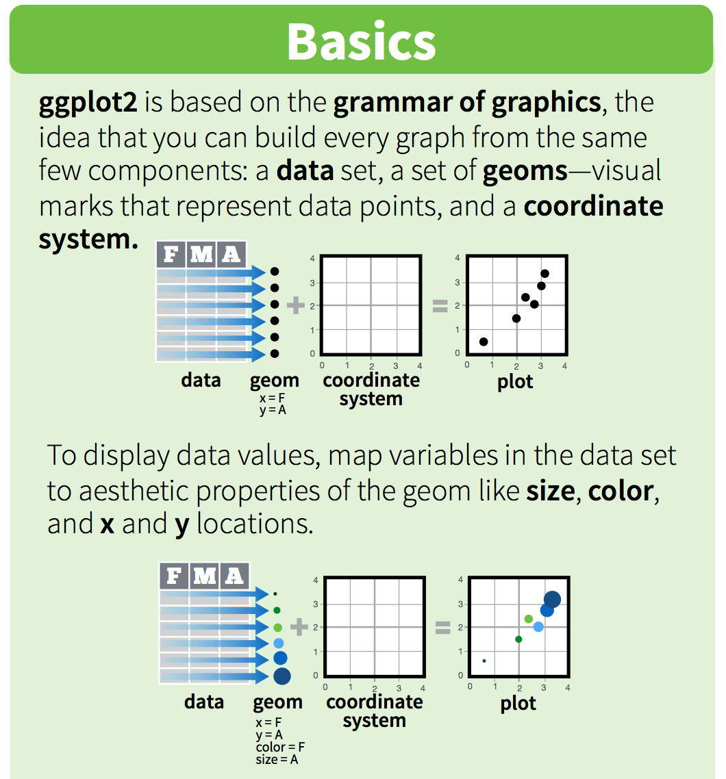
These “same few components” that all ggplot2 graphs
share include the followings:
Of these, data, aesthetics, and geometries are the components that must be specified when creating a graph.
From STAT545:
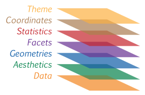
You can think of the grammar of graphics as a systematic approach for
describing the components of a graph. It has seven components (the ones
in bold are required to be specifed explicitly in
ggplot2):
Required:
- Data
- Exactly as it sounds: the data that you’re feeding into a plot.
- Aesthetic mappings
- This is a specification of how you will connect variables (columns) from your data to a visual dimension. These visual dimensions are called “aesthetics”, and can be (for example) horizontal positioning, vertical positioning, size, colour, shape, etc.
- Geometric objects
- This is a specification of what object will actually be drawn on the plot. This could be a point, a line, a bar, etc.
Optional:
- Scales
- This is a specification of how a variable is mapped to its aesthetic. Will it be mapped linearly? On a log scale? Something else?
- Statistical transformations
- This is a specification of whether and how the data are combined/transformed before being plotted. For example, in a bar chart, data are transformed into their frequencies; in a box-plot, data are transformed to a five-number summary.
- Coordinate system
- This is a specification of how the position aesthetics (x and y) are depicted on the plot. For example, rectangular/cartesian, or polar coordinates.
- Facet
- This is a specification of data variables that partition the data into smaller “sub plots”, or panels.
These components are like parameters of statistical graphics, defining the “space” of statistical graphics. In theory, there is a one-to-one mapping between a plot and its grammar components, making this a useful way to specify graphics.
We will use the ggplot2 package, but the function we use
to initialize a graph will be ggplot, which works best for
data in tidy format (i.e., a column for every variable, and a row for
every observation). We will learn more about the tidy format and how to
convert “untidy” datasets into tidy format later in the class. For the
next few lectures, the datasets that we will use are already in tidy
format.
Graphics with ggplot2 are built step-by-step, adding new
elements as layers with a plus sign (+) between layers.
Adding layers in this fashion allows for extensive flexibility and
customization of plots. Below is a template that can be used to create
almost any graph that you can imagine using ggplot2.
ggplot(data = <DATA>) +
  <GEOM_FUNCTION>(
     mapping = aes(<MAPPINGS>),
     stat = <STAT>,
     position = <POSITION>
  ) +
  <COORDINATE_FUNCTION> +
  <FACET_FUNCTION> +
  <THEME_FUNCTION>
Breaking that down:
- First, tell R you are using
ggplot()
- Then, tell it the object name under which your data table is stored
(
data = <DATA>)
- Next, add a layer for the type of geometric object with
<GEOM_FUNCTION>. For example, geom_point() generates a scatterplot, geom_line() generates a line graph, geom_bar() generates a bar graph, etc.
- Then, use
mapping = aes(<MAPPINGS>)to specify which variables you want to plot in this layer and which aesthetics they should map to. - (Optional) Use
stat = <STAT>to perform statistical transformation with your variables. - (Optional) Use
position = <POSITION>to perform any position adjustment with your geometric object. - (Optional) Use
<COORDINATE_FUNCTION>to change the default coordinate system. - (Optional) Use
<FACET_FUNCTION>to make a faceted graph. - (Optional) Use
<THEME_FUNCTION>to change the default style of the graph.
A simple scatter plot
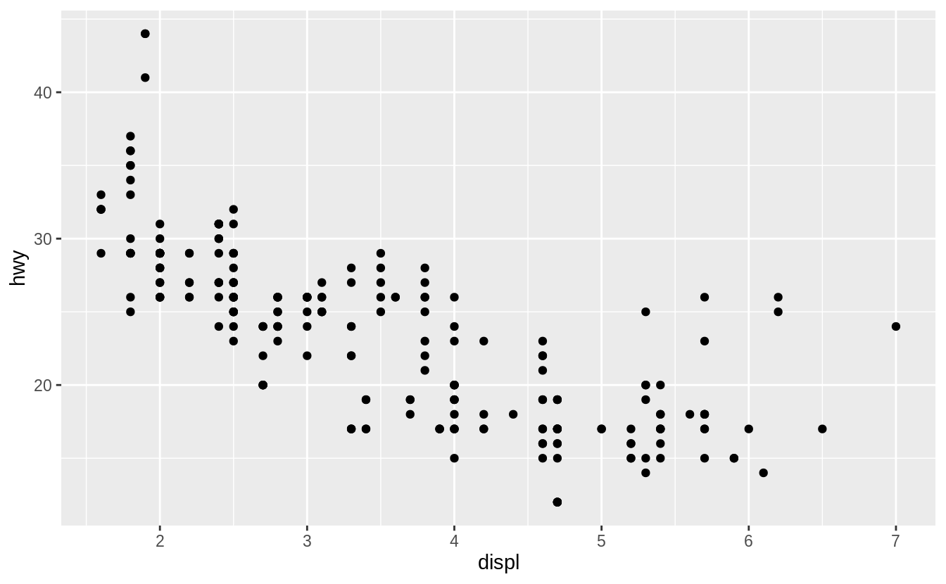
Let’s first make a simple scatter plot to look at how engine
displacement (displ), which is an expression of an engine’s
size, may affect the fuel economy of cars on the highway
(hwy). For this plot, what are the aesthetics, and what are
the geometric objects?
We can make this plot by entering the relevant data,
geom_function and mappings in the general ggplot template.
ggplot(data = <DATA>) +
  <GEOM_FUNCTION>(mapping = aes(<MAPPINGS>))
In our case, it would be
## demo
ggplot(data = mpg) +
geom_point(mapping = aes(x = displ, y = hwy)) 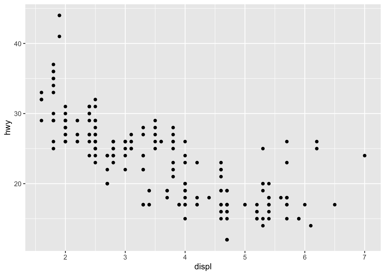
Your turn - Exercise 2
Run
ggplot(data = mpg). What do you see? Why?Make a scatterplot of
hwyvscylIf you have time, see what happens if you make a scatterplot of
classvsdrv? Why is the plot not useful?
Make the size of points correspond to the number of cylinders
(cyl), and the color of points corresponds to the type of
car (class)
The scatter plot shows that there is a negative correlation between engine size and fuel economy. However, there are a few points that show up as outliers from this general trend. Why might this be?
To explore this further, we will map cyl to
size, and class to color.
## demo
ggplot(data = mpg) +
geom_point(mapping = aes(x = displ, y = hwy, color = class, size = cyl)) 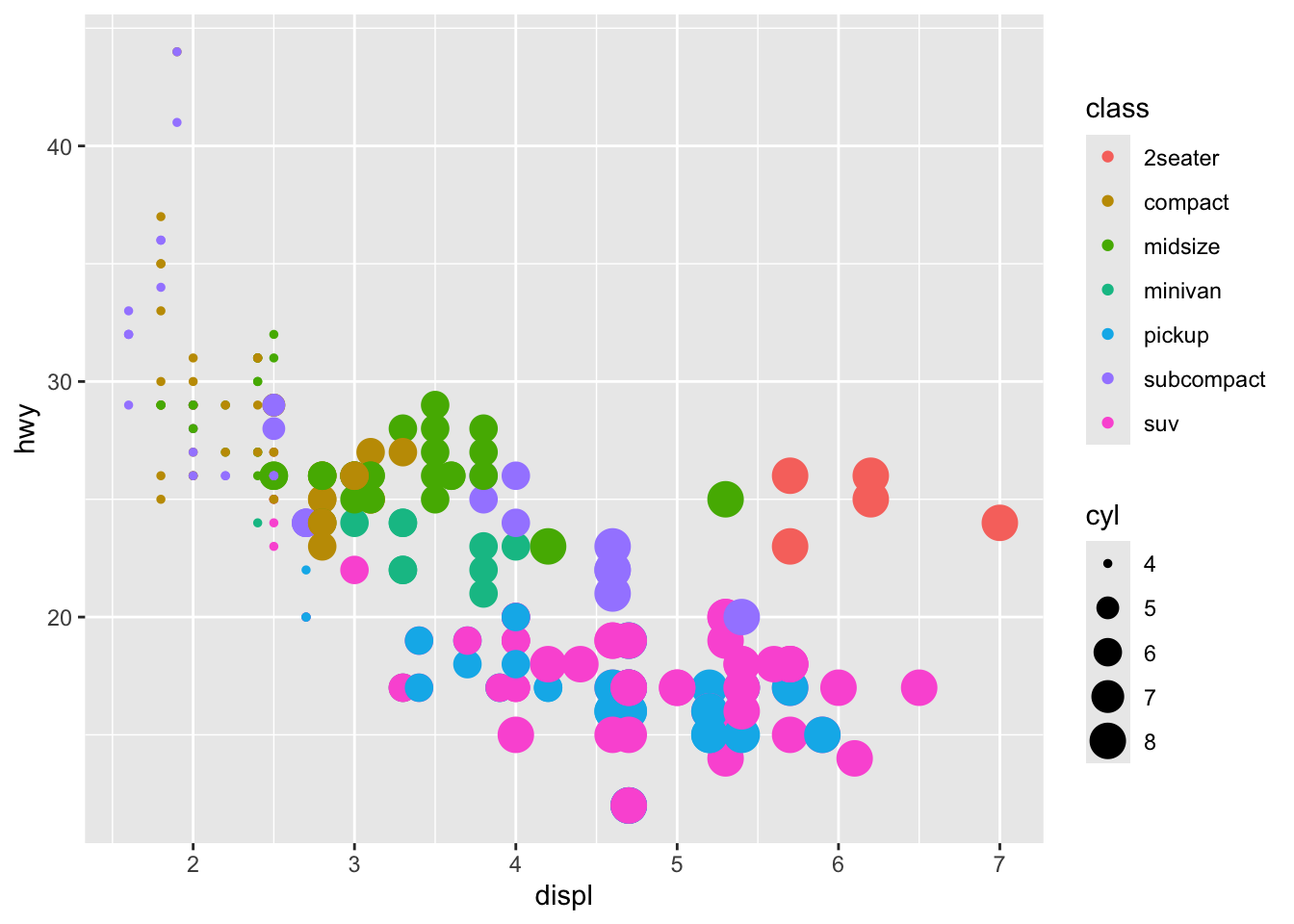
It looks like given the same engine size, 2seaters tend to have better fuel economy than other car types. This makes sense.
Change the shape of all points
There is too much overlap among the larger points in the previous
graph and we want to use a different point shape (shape) to
show these points more clearly. When all points in the graph get the
same aesthetic, we are no longer mapping the aesthetic to a variable.
Therefore, we should make sure to specify this outside of the
mapping argument.
## demo (change point shape to 1)
ggplot(data = mpg) +
geom_point(mapping = aes(x = displ, y = hwy, color = class, size = cyl), shape = 1) 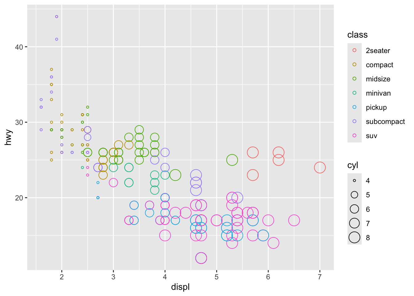
Your turn - Exercise 3
Return to your scatterplot of
hwyvscyl. Color the points by the year of manufacture for each car model. Why does the legend look different from when we mappedclassto color above?Next make a similar plot in which you color all the points blue
If you have time, figure out what has gone wrong with this plot. Why are the points not blue?
ggplot(data = mpg) +
  geom_point(mapping = aes(x = displ, y = hwy, color = "blue"))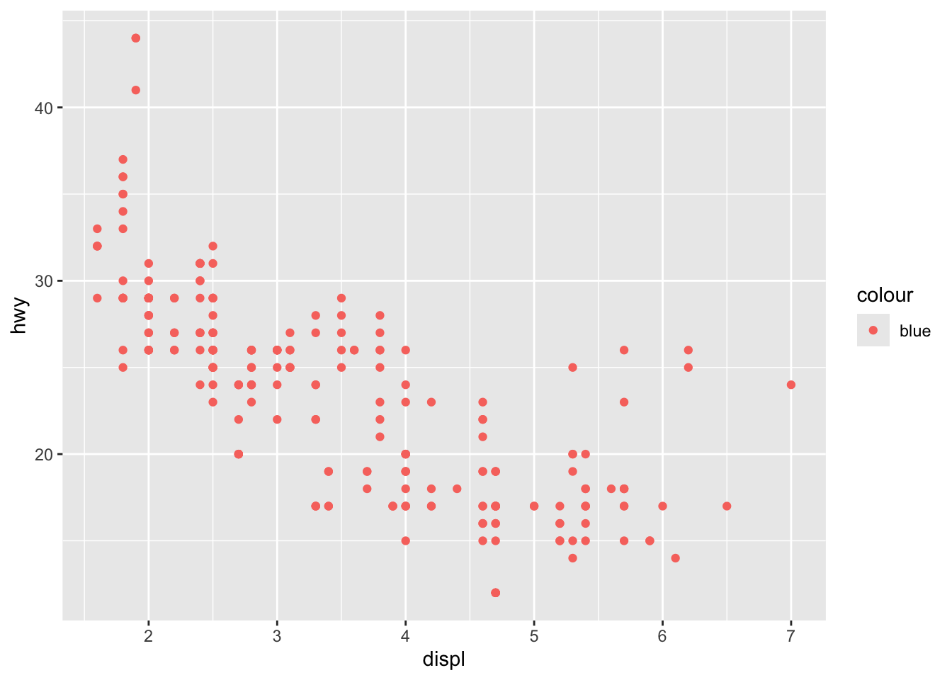
Save your note file and sync your project with your GitHub repo.
Overlay two different geometric objects
Here, we will add a trend line to the scatter plot above. We can do
this by adding another geometric object (geom_smooth()) on
top of the previous graph. Give it a try yourself first.
## exercise, then demo
ggplot(data = mpg) +
  geom_point(mapping = aes(x = displ, y = hwy, color = class, size = cyl), shape=1) +
  geom_smooth(mapping = aes(x = displ, y = hwy))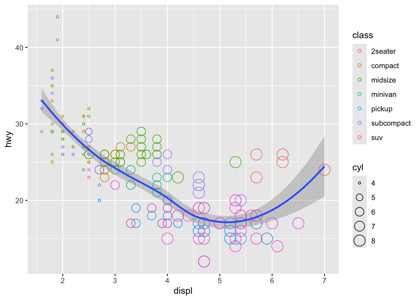
Did you notice that for both geometric objects, x maps
to displ and y maps hwy, so these
auguments are repeated? In such cases, we can minimize the amount of
repeat by defining how these aesthetics map to variables for all
subsequent layers within ggplot(), as the following.
## demo
ggplot(data = mpg, mapping = aes(x = displ, y = hwy)) +
  geom_point(mapping = aes(color =class, size = cyl), shape = 1) +
  geom_smooth()
Display different year in different facets
One way to add additional variables is with aesthetics. Another way, particularly useful for categorical variables, is to split your plot into facets, subplots that each display one subset of the data.
The mpg dataset contains cars made in 1999 and 2008. To
check whether the relationship between displ and
hwy remains the same across time, we can add a facet
function to the previous plot and plot the two years side by side.
## demo
ggplot(data = mpg, mapping = aes(x = displ, y = hwy)) +
  geom_point(mapping = aes(color = class, size = cyl), shape = 1) +
  geom_smooth() +
  facet_wrap(~ year, nrow=1)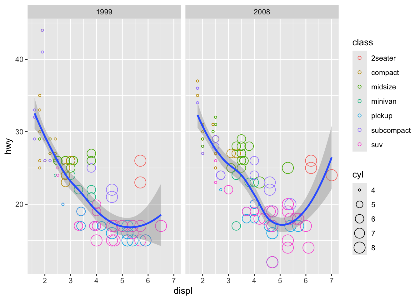
Your turn - Exercise 4
Break this plot into subplots for each class
ggplot(data = mpg) +
  geom_point(mapping = aes(x = displ, y = hwy))
Adjust figure size using chunk options
Note that each facet in the figure above appears to be quite narrow.
To make the figure wider, use Quarto chunk options
fig.height and fig.width, e.g. starting your
code chunk with ```{r fig.height=5, fig.width=10}.
## demo
ggplot(data = mpg, mapping = aes(x = displ, y = hwy)) +
  geom_point(mapping = aes(color = class, size = cyl), shape = 1) +
  geom_smooth() +
  facet_wrap(~ year, nrow=1)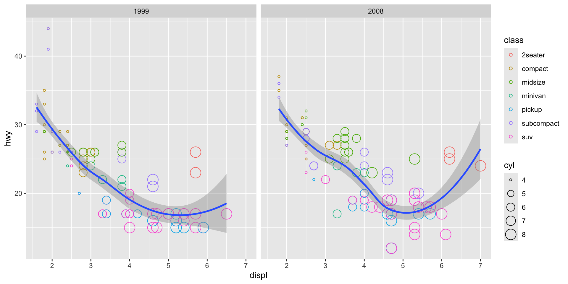
Change the theme of a graph
While every element of a ggplot2 graph is customizable,
there are also built-in themes (theme_*()) that you can use
to make some major headway before making smaller tweaks manually. Let’s
try one of them here. You can look at other built-in themes here.
## demo (use theme_bw)
ggplot(data = mpg, mapping = aes(x=displ, y=hwy)) +
  geom_point(mapping = aes(color=class, size=cyl), shape=1) +
  geom_smooth() +
  facet_wrap(~ year, nrow=1) +
  theme_bw()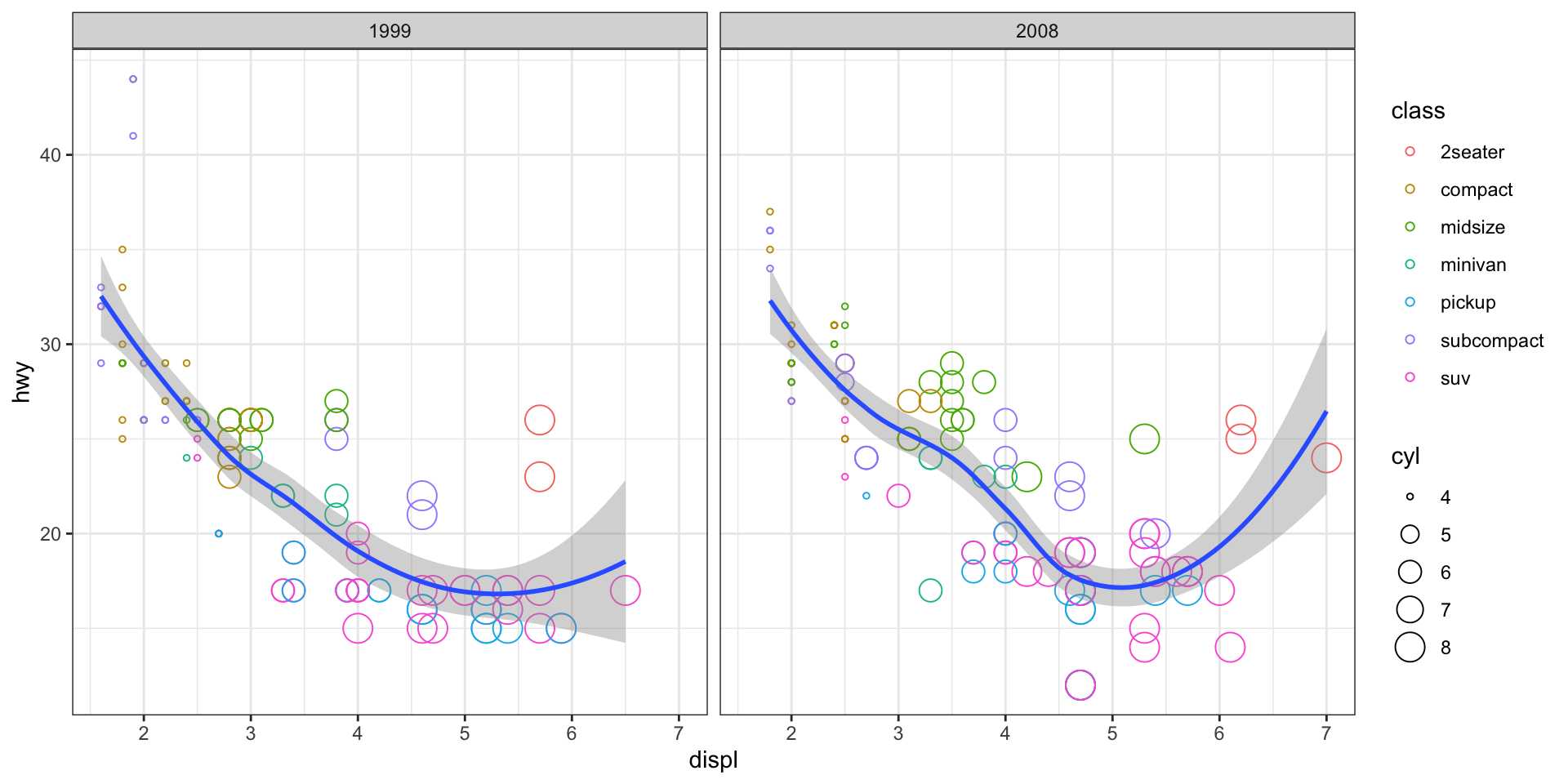
Arguments and functions that are nice know
Now, you’ve learned the central ideas behind ggplot2. In
our next ggplot2 lecture, we will go over some more
advanced ggplot2 functionalities (e.g. statistical transformation,
position adjustment, coordinate setting, color scaling, theme), but
after that, the best way to learn more about ggplot2 is
often through practice and Google, since the possibilities that you can
have with ggplot2 are quite limitless, and people’s
plotting needs vary.
That being said, there are some geometries, aesthetics, and facet functions that are most commonly used and these often serve as the building blocks for more advance usage. Let’s now go through some of these together in class. The RStudio ggplot cheatsheet is a great resource for looking up other functionality.
Geometries
geom_point()
geom_boxplot()## exercise, then demo (hwy vs. class) ggplot(data = mpg) + geom_boxplot(mapping = aes(x = class, y = hwy))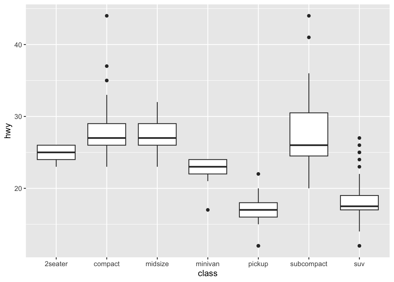
geom_bar()## exercise, then demo (class) ggplot(mpg) + geom_bar(mapping = aes(x = class))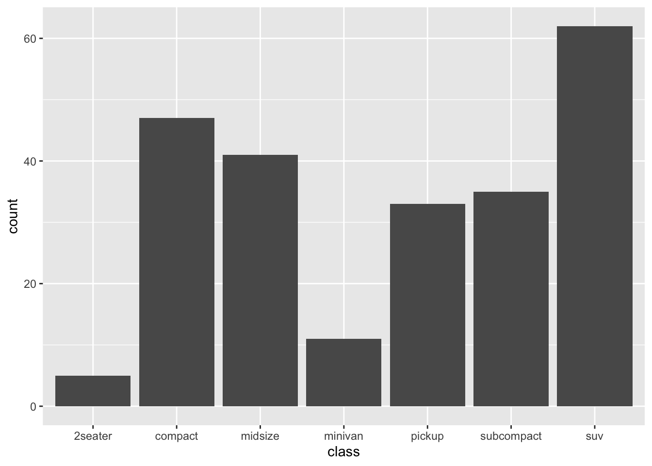
geom_histogram()## exercise, then demo (hwy) ggplot(mpg) + geom_histogram(mapping = aes(x = hwy))## `stat_bin()` using `bins = 30`. Pick better value with `binwidth`.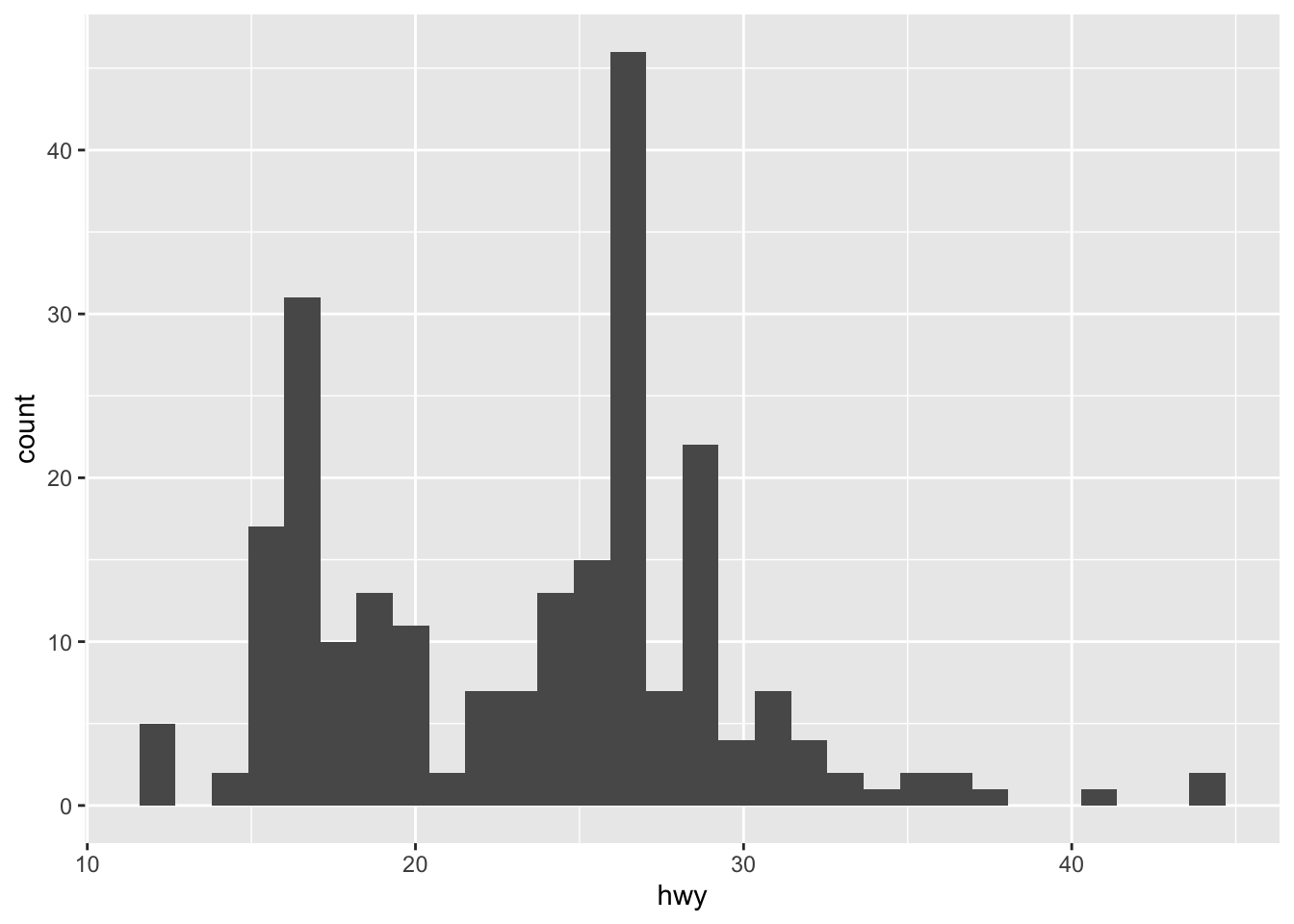
geom_density()## exercise, then demo (hwy) ggplot(mpg) + geom_density(mapping = aes(x = hwy))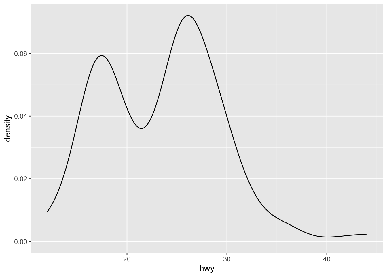
geom_smooth()Different
geom_*()functions have different arguments that can be very helpful. You can learn more about them by reading their help pages. For example,method="lm"andse=FALSEare two arguments that are often used in thegeom_smooth()function.## exercise, then demo (fit linear model to hwy vs. displ without confidence interval) ggplot(mpg, aes(x = displ, y = hwy))+ geom_point() + geom_smooth(method = "lm", se = F)## `geom_smooth()` using formula = 'y ~ x'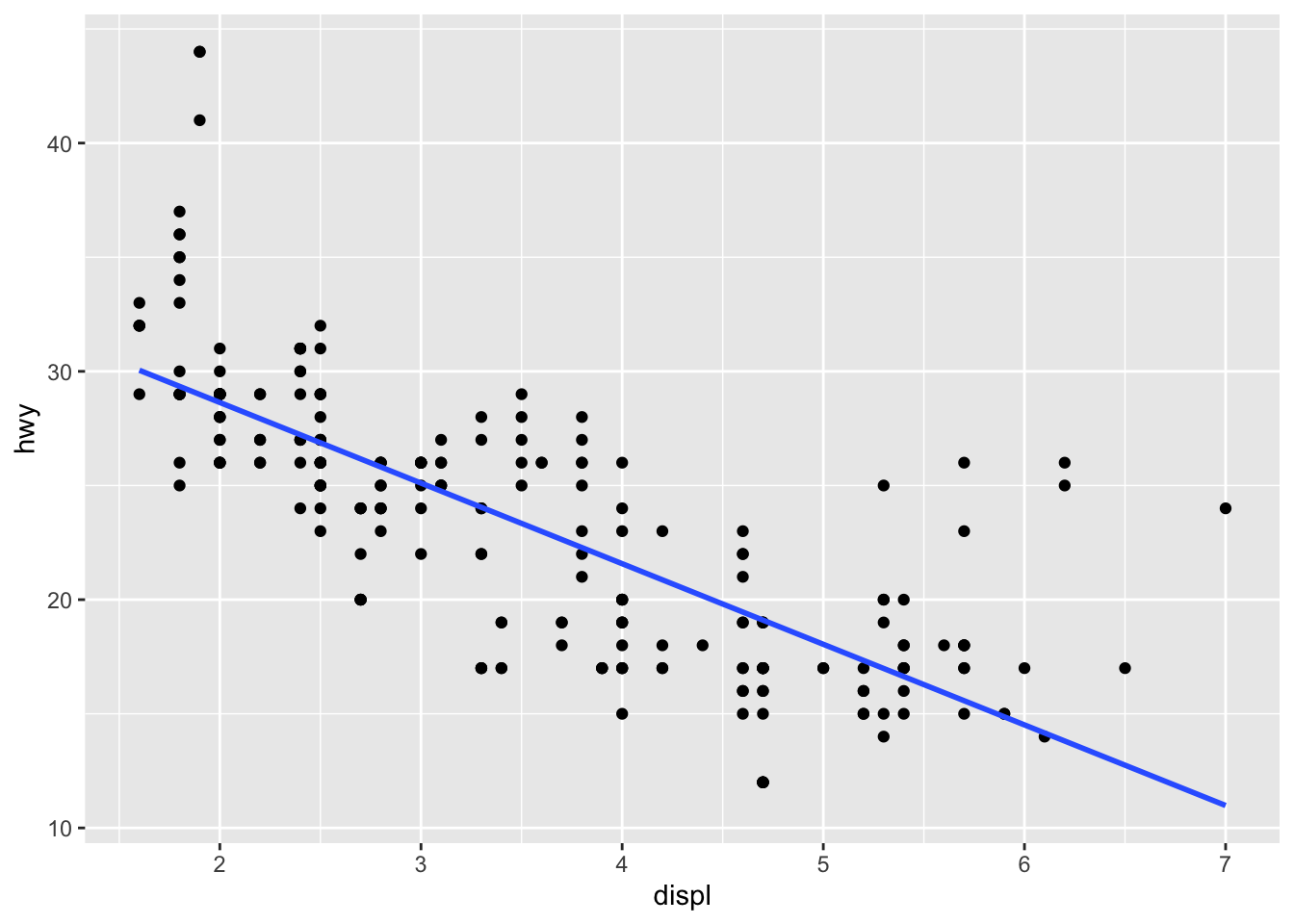
geom_text()## demo (hwy vs. displ, cyl as the label) ggplot(mpg, aes(x = displ, y = hwy))+ geom_text(mapping = aes(label = cyl))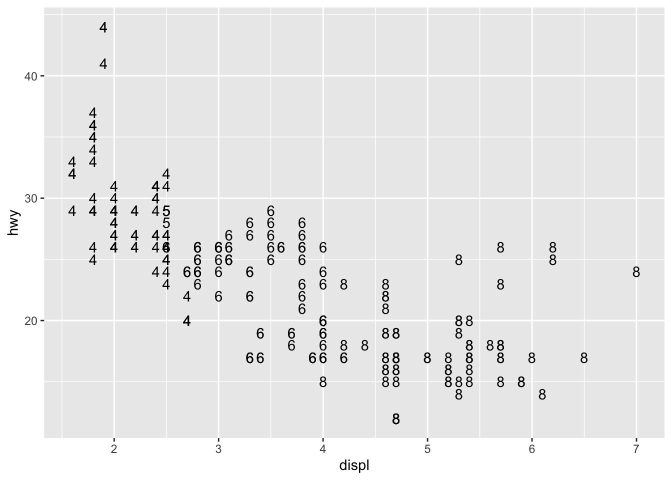
geom_label()Each geometric object can take a different data frame if specified. Here is an example of that.
## demo (hwy vs. displ, model as the label but only label points with hwy > 40)
ggplot(mpg)+
  geom_point(aes(x = displ, y = hwy)) +
  geom_label(data = filter(mpg, hwy > 40), mapping = aes(label = model, y = hwy, x = displ + 0.4))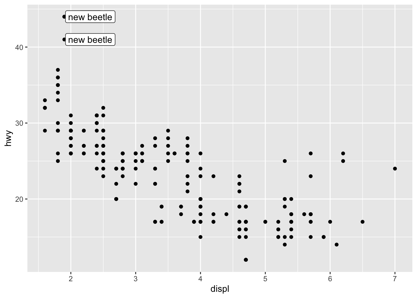
geom_line()## demo (change in mean hwy for each car model over time, grouped by model, colored by class, faceted by manufacturer) group_by(mpg, manufacturer, year, class, model) %>% summarize(mean_hwy = mean(hwy)) %>% ggplot(aes(x = year, y = mean_hwy, color = class, group = model)) + geom_point() + geom_line() + facet_wrap(~ manufacturer)## `summarise()` has grouped output by 'manufacturer', 'year', 'class'. You can ## override using the `.groups` argument.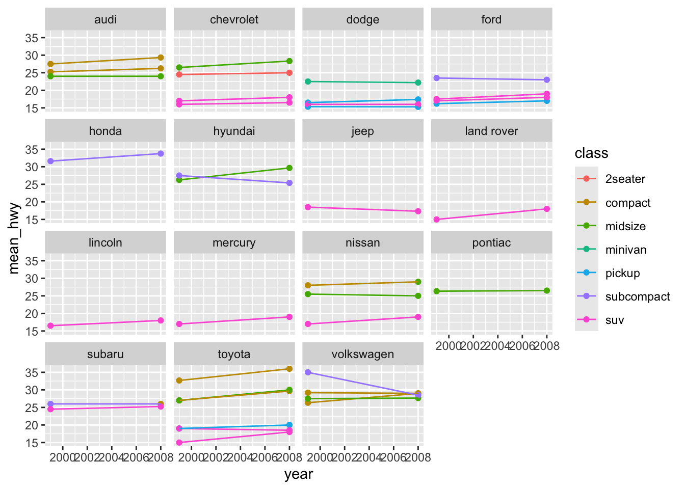
Aesthetics
x,ysizelabelgroupcolor,fill(colorcontrols the color of points and lines, whereasfillcontrols the color of surfaces)## demo (plot hwy distribution with geom_density, color by drv) ggplot(mpg) + geom_density(aes(color = drv, x = hwy))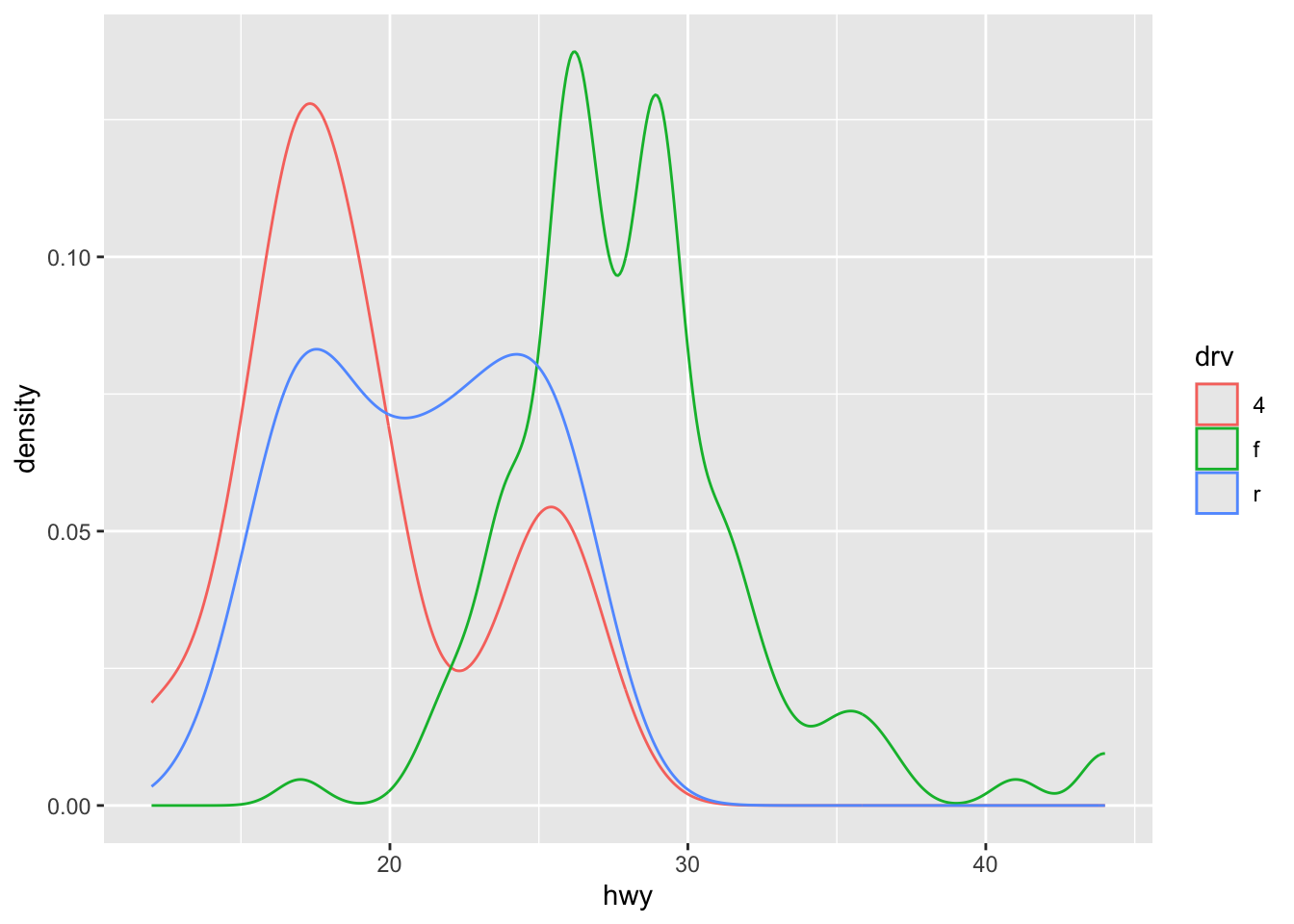
## demo (fill by drv)
ggplot(mpg) +
  geom_density(aes(fill = drv, x = hwy))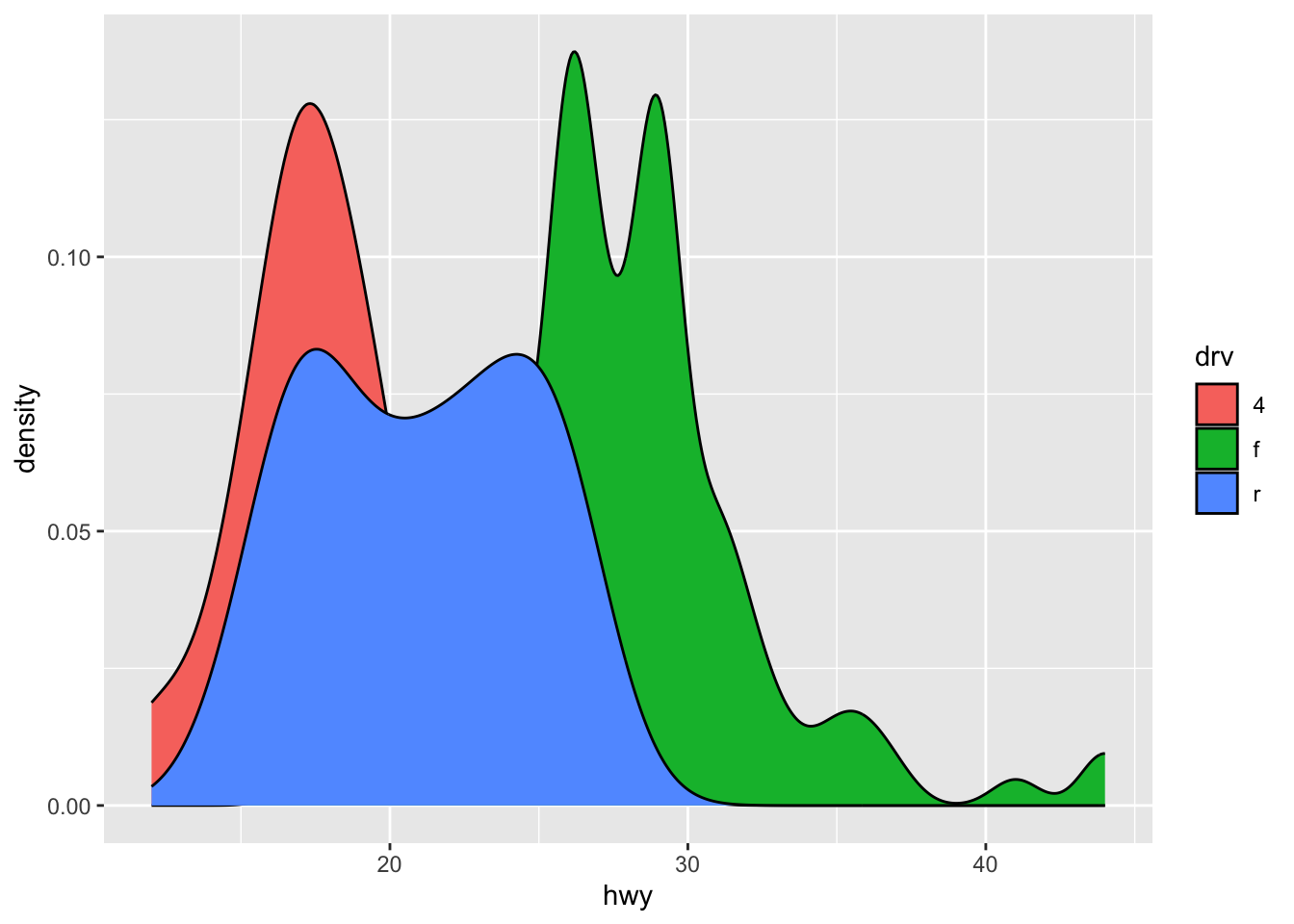
alphaalphacontrols tranparency## demo (plot hwy distribution with geom_density, fill by drv, set alpha to 0.5) ggplot(mpg) + geom_density(aes(fill = drv, x = hwy), alpha = 0.5)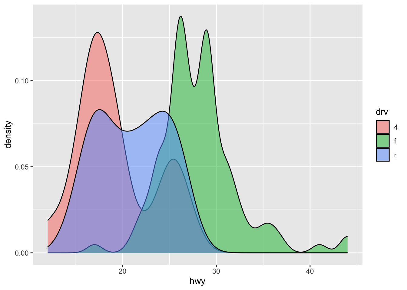
shape,line_type## demo (hwy vs. displ, geom_point and geom_line, map drv to color, shape, linetype) ggplot(mpg, aes(x = displ, y = hwy, color = drv, shape = drv)) + geom_point()+ geom_smooth(aes(linetype = drv))## `geom_smooth()` using method = 'loess' and formula = 'y ~ x'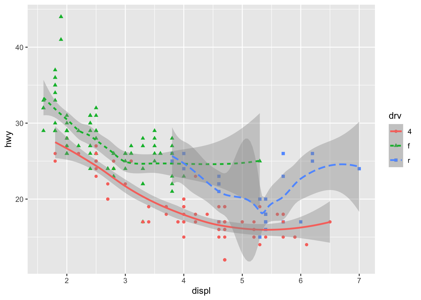
Facet
facet_wrap()facet grid()## demo (hwy vs displ, faceted by cyl and drv) ggplot(mpg, aes(x = displ, y = hwy)) + geom_point() + facet_grid(drv ~ cyl)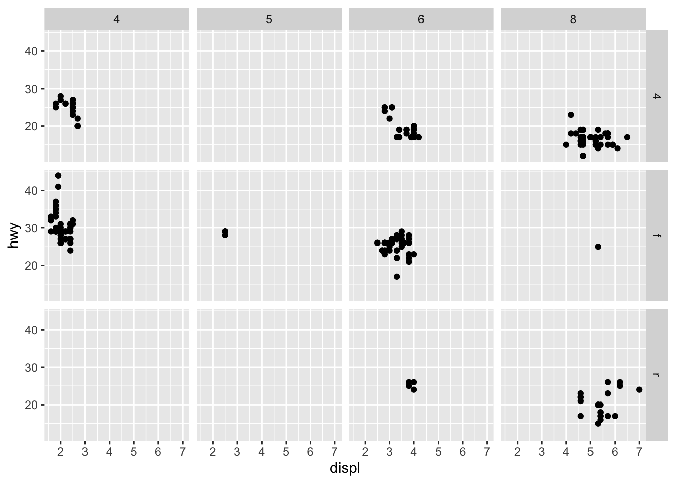
Exporting a ggplot graph with ggsave()
If we want our graph to appear in a knitted html, then we don’t need to do anything else. But often we’ll need a saved image file, of specific size and resolution, to share or for publication.
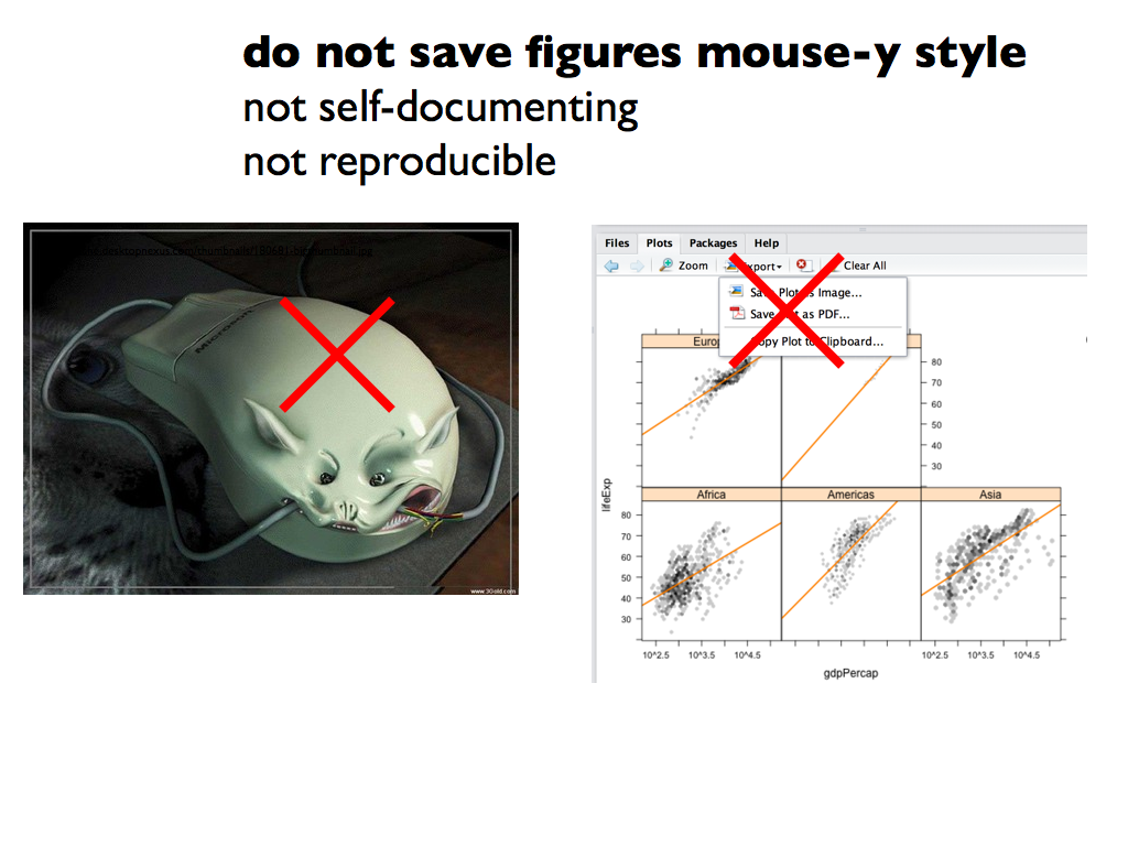 Graphic
from Jenny
Bryan’s ggplot tutorial
Graphic
from Jenny
Bryan’s ggplot tutorial
ggsave() will export the most recently run
ggplot graph by default (plot = last_plot()), unless you
give it the name of a different saved ggplot object.
It has smart defaults and guesses the format from the file extension name (you can use e.g. pdf, tiff, eps, png, mmp, svg). It doesn’t force you to do annoying things with dots per inch etc (but you can if you want to).
Some common arguments for ggsave():
width =: set exported image width (default inches)height =: set exported image height (default height)dpi =: set dpi (dots per inch)
For more details on how to use ggsave() see slides 50-56
in Jenny
Bryan’s ggplot tutorial
Example ggsave() options
If the plot is on your screen
ggsave("path_to_figure/filename.png")If your plot is assigned to an object
ggsave(filename = "path_to_figure/filename.png", plot1)Specify a size
ggsave(filename = "path_to_figure/filename.png", width = 5, height = 3)Or any format (pdf, png, eps, jpp, svg)
ggsave(filename = "path_to_figure/filename.png")
ggsave(filename = "path_to_figure/filename.pdf")
ggsave(filename = "path_to_figure/filename.jpg")
Now we’re done for today
Save your scripte and sync your project with your GitHub repo.
- Save
- Stage
- Commit
- Pull (to check for remote changes)
- Push!